[NOTE: This is a repost of a blog that Prasanna Parasurama published at the blogsite Towards Data Science].

“The confidence intervals of the two groups overlap, hence the difference is not statistically significant” 

The statement above is wrong. Overlapping confidence intervals/error bars say nothing about statistical significance. Yet, a lot of people make the mistake of inferring lack of statistical significance. Likely because the inverse — non-overlapping confidence intervals — means statistical significance. I’ve made this mistake. I think part of the reason it is so pervasive is that it is often not explained why you cannot compare overlapping confidence intervals. I’ll take a stab at explaining this in this post in an intuitive way. HINT: It has to do with how we keep track of error.

The Setup

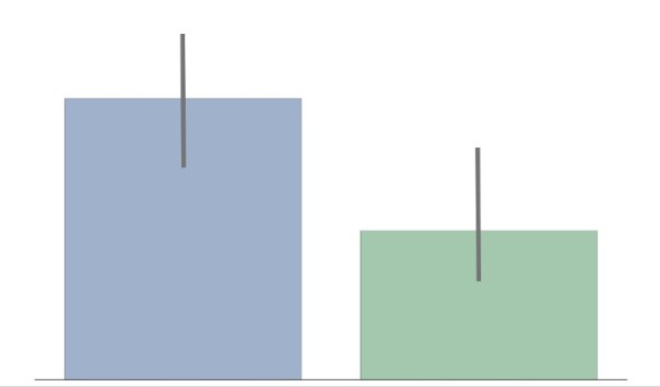
– We have 2 groups:  Group Blue and Group Green.

– We are trying to see if there is a difference in age between these two groups.

– We sample the groups to find the mean μ, and standard deviation σ (aka error) and build a distribution: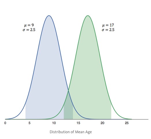– Group Blue’s average age is 9 years with an error of 2.5 years. Group Green’s average age is 17, also with an error of 2.5 years.

– The shaded regions show the 95% confidence intervals (CI).

From this setup, many will erroneously infer that there is no statistical significant difference between groups, which may or may not be correct.

The Correct Setup

– Instead of building a distribution for each group, we build one distribution for the difference in mean age between groups.

– If the 95% CI of the difference contains 0, then there is no difference in age between groups. If it doesn’t contain 0, then there is a statistically significant difference between groups.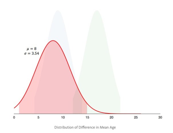As it turns out the difference is statistically significant, since the 95% CI (shaded region) doesn’t contain 0.

Why?

In the first setup we draw the distributions, then find the difference. In the second setup, we find the difference, then draw the distribution. Both setups seem so similar, that it seems counter-intuitive that we get completely different outcomes. The root cause of the difference lies in error propagation — fancy way of saying how we keep track of error.

Error Propagation

Imagine you are trying to measure the area A of a rectangle with sides L, W. You measure the sides with a ruler and you estimate that there is an error of 0.1 associated with measuring a side.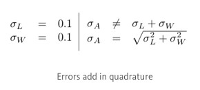To estimate the error of the area, intuitively you’d think it is 0.1 + 0.1 = 0.2, because errors add up. It is almost correct; errors add, but they add in quadrature (squaring then taking the square root of the sum). That is, imagine these errors as 2 orthogonal vectors in space. The resulting error is the magnitude of sum of these vectors.

Circling Back

The reasons we get different results from the 2 setups is how we propagate the error for difference in age.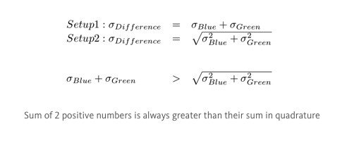In the first setup, we simply added the errors of each group. In the second setup, we added the errors in quadrature. Since adding in quadrature will yield a smaller value than adding normally, we overestimated the error in the first setup, and incorrectly inferred no statistical significance.