[* EiR = Econometrics in Replications, a feature of TRN that highlights useful econometrics procedures for re-analysing existing research.]

NOTE: All the data and code  necessary to produce the results in the tables below are available at Harvard’s Dataverse: click here.

Fixed effects estimators are often used when researchers are concerned about omitted variable bias due to unobserved, time-invariant variables. These can prove insightful if there is much within-variation to support the fixed effects estimate. However, they can be misleading when there is not.

Stata has several commands that can help the researcher gauge the extent of within-variation. In this example, we use the “wagepan” dataset that is bundled with Jeffrey Wooldridge’s text, “Introductory Econometrics: A Modern Approach, 6e”. The dataset consists of annual observations of 545 workers over the years 1980-1987. It is described here.

In this example we use fixed effects to regress log(wage) on education, labor market experience, labor market experience squared, dummy variables for marital and union status, and annual time dummies.

The table below reports the fixed effects (within-estimate) for the “married” variable. For the sake of comparision, it also reports the between-estimate for “married” (calculated used the Mundlak version of the Random Effects Within Between estimator (Bell, Fairbrother, and Jones, 2019).

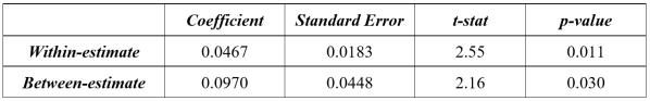
The within-estimate of the marriage premium is smaller than the between-estimate. This is consistent with marital status being positively associated with unobserved, time-invariant productivity characteristics of the worker. However, we want to know how much variation there is in marital status for the workers in our sample. If it is just a few workers who are changing marital status over time, then our estimate may not be representative of the effect of marriage in the population.

Stata provides two commands that can be helpful in this regard. The command xttab reports, among other things, a measure of variable stability across time periods. In the table below, among workers who ever reported being unmarried, they were unmarried for an average of 64.8% of the years in the sample.

Among workers who ever reported being married, they were married for 62.5% of the years in the sample. In this case, changes in marital status are somewhat common. Note that a time-invariant variable would have a “Within Percent” value of 100%.

Stata provides another command, xttrans, that gives detail about year-to-year variable transitions.

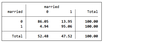
The rows represent the values in year t, with the columns representing the values in the following year. In this case, 86% of observations that were unmarried at time t, were also unmarried at time t+1. 14% of observations that were unmarried at time t changed status to “married” at time t+1.

Among other things, the xttrans command provides a reminder that the fixed effects estimate of the marriage premium includes the effect of transitioning from married to unmarried: 5% of observations that were married at time t were unmarried at time t+1. The implied assumption is that the effect of marriage on wages is symmetric, something that could be further explored in the data.

While these analyses are useful, they are based on observations, not workers. If there is concern about sample selection biasing the fixed effects estimates (so that “movers” are different from “stayers”), it would be useful to know how many of the 545 workers had experienced a marital status change, since it is the changes that support the fixed effects estimate.

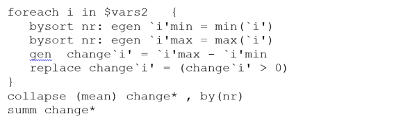
The following set of commands calculate the min and the max values of the explanatory variables for all the workers in the sample. It then creates a dummy variable with the prefix “change” that takes the value 1 anytime the max and min values differ. Finally, it collapses the dataset so that there is one observation per worker, and then takes averages of the change variables.

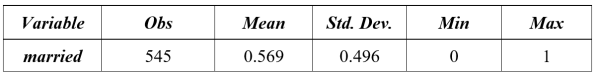
The results below indicate that 56.9% of the workers changed their marital status during the sample period. Whether this is a sufficient number of “changers” to represent population “changers” is an open question. However, if the number were only 5 or 10% of workers, the argument for representativeness would be much weaker.

What does this have to do with replication? Oftentimes treatments are administered over time in panel datasets (say microcredit loans). Fixed effects estimates may be used to identify causal estimates of the treatment. Sample statistics, when they are reported, typically only report the percent of observations receiving treatment. Consider the two samples below.

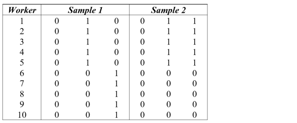
In both samples, 30% of the observations are treatment observations. Thus a table of sample statistics would show identical means for the treatment variable in the two samples.

However, in the first sample, 100% of the workers received treatment, and 75% of year-to-year transitions involved a change in treatment status. In the second sample, only 50% of the workers experienced treatment, and 25% of year-to-year transitions involved a change in treatment status.

These are the kinds of differences that the procedures described above can be used to identify.

Bob Reed is a professor of economics at the University of Canterbury in New Zealand. He is also co-organizer of the blogsite The Replication Network. He can be contacted at bob.reed@canterbury.ac.nz.