An estimated 85% of global health research investment is wasted (Chalmers and Glasziou, 2009); a total of one hundred billion US dollars in the year 2009 when it was estimated. The movement to reduce this research waste recommends that previous study results be taken into account when prioritising, designing and interpreting new research (Chalmers et al., 2014; Lund et al., 2016). Yet any recommendation to increase efficiency this way requires that researchers evaluate whether the studies already available are sufficient to complete the research effort; whether a new study is necessary or wasteful. These decisions are essentially stopping rules – or rather noisy accumulation processes, when no rules are enforced – and unaccounted for in standard meta-analysis. Hence reducing waste invalidates the assumptions underlying many typical statistical procedures.

Ter Schure and Grünwald (2019) detail all the possible ways in which the size of a study series up for meta- analysis, or the timing of the meta-analysis, might be driven by the results within those studies. Any such dependency introduces accumulation bias. Unfortunately, it is often impossible to fully characterize the processes at play in retrospective meta-analysis. The bias cannot be accounted for. In this blog we revisit an example accumulation bias process, that can be one of many influencing a single meta-analysis, and use it to illustrate the following key points:

– Standard meta-analysis does not take into account that researchers decide on new studies based on other study results already available. These decisions introduce accumulation bias because the analysis assumes that the size of the study series is unrelated to the studies within; it essentially conditions on the number of studies available.

– Accumulation bias does not result from questionable research practices, such as publication bias from file-drawering a selection of results. The decision to replicate only some studies instead of all of them biases the sampling distribution of study series, but can be a very efficient approach to set priorities in research and reduce research waste.

– ALL-IN meta-analysis stands for Anytime, Live and Leading INterim meta-analysis. It can handle accumulation bias because it does not require a set number of studies, but performs analysis on a growing series – starting from a single study and accumulating as many studies as needed.

– ALL-IN meta-analysis also allows for continuous monitoring of the evidence as new studies arrive, even as new interim results arrive. Any decision to start, stop or expand studies is possible, while keeping valid inference and type-I error control intact. Such decisions can be strategic: increasing the value of new studies, and reducing research waste.

Our example: extreme Gold Rush accumulation bias

We imagine a world in which a series of studies is meta-analyzed as soon as three studies become available. Many topics deserve a first initial study, but the research field is very selective with its replications. Nevertheless, for significant results in the right direction, a replication is warranted. We call this the Gold Rush scenario, because after each finding of a positive significant result – the gold in science – some research group rushes into a replication, but as soon as a study disappoints, the research effort is terminated and no-one bothers to ever try again. This scenario was first proposed by Ellis and Stewart (2009) and formulated in detail and under this name by Ter Schure and Grünwald (2019). Here we consider the most extreme version of the Gold Rush where finding a significant positive result not only makes a replication more probable, but even inevitable: the dependency of occurring replications on their predecessor’s result is deterministic.

Biased Gold Rush sampling

We denote the number of studies available on a certain topic by t. This number t can also indicate the timing of a meta-analysis, such that a meta-analysis can possibly occur at number of studies t = 1, 2, 3, . . . up to some maximum number of studies T . This notation follows from Ter Schure and Grünwald (2019); the Technical Details at the end of this blog make the notation involved in this blog more explicit.

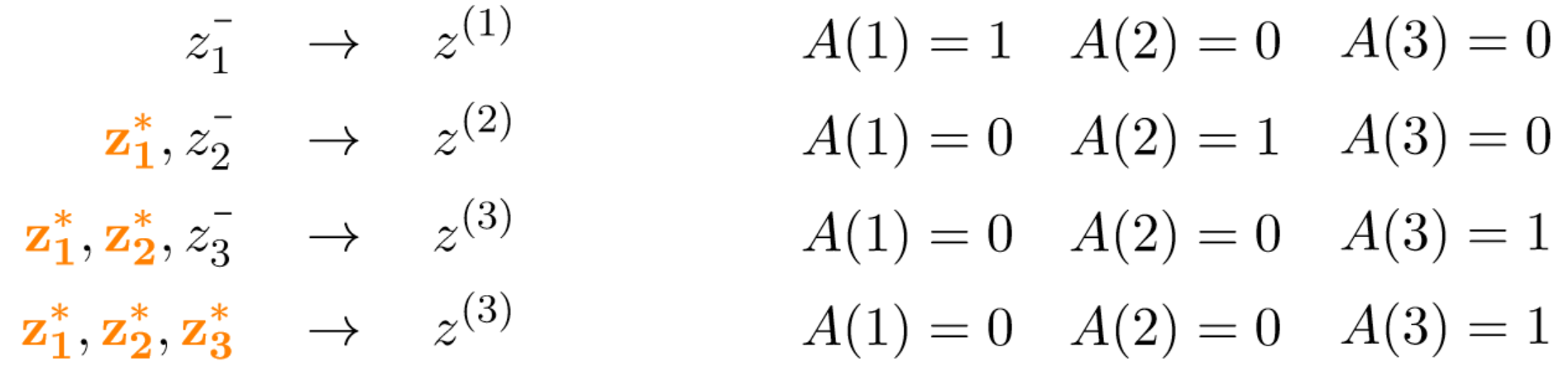
We summarize the results of individual studies into a single per-study Z-score (z₁ for the first study, z₂ for the second, etc), such that we have the following information on a series of size t: z₁, z₂, . . . , z_t . We distinguish between Z-scores that are significant and in the right direction, and Z-scores that are not. A first significant positive study is indicated by z₁ = z₁*   (z₁* > z_α with z_α = 1.96 for α = 2.5%).  A first nonsignificant or negative study is indicated by z₁ = z₁^– (z₁ <= z_α).  We use the same notation for the second and third study and limit our world to three studies (our maximum T = 3). After all, we meta-analyze studies on all topics and only those topics that have spurred a series of three studies. Our Gold Rush world consists of the following possible study series:

Gold Rush world

Here A(t) denotes whether we accumulate and analyze the t studies: It can be that A(2) = 0 and A(3) = 0 because we are stuck at one study, but also A(1) = 0 because we don’t “meta-analyze” that single study. It can only be that A(2) = 1 if we accumulate and meta-analyze a two-study series and A(3) = 1 if we accumulate and meta-analyze a three-study series. In our Gold Rush world a very specific subset of studies accumulate into a three-study series such that they are meta-analyzed (A(3) = 1).

z⁽³⁾ denotes the Z-score of a fixed effects meta-analysis. This meta-analysis Z-score is simply a re-normalized average and can, assuming equal sample size and variances in all studies, be obtained from the individual study  Z-scores  as  follows: z⁽³⁾ =[1/sqrt(3)) × sum(z_i)_{i = 1 to 3}]. The effects of accumulation bias are not limited to fixed-effects meta-analysis (see for example Kulinskaya et al. (2016)), but fixed-effects meta-analysis does provide us with a simple illustration for the purposes of this blog.

We observe in our Gold Rush world above that the study series that are eventually meta-analyzed into a Z-score z⁽³⁾ are a very biased subset of all possible study series. So we expect these z⁽³⁾ scores to be biased as well. In the next section, we simulate the sampling distribution of these z⁽³⁾ scores to illustrate this bias.

The conditional sampling distribution under extreme Gold Rush accumulation bias

Assume that we are in the scenario that only true null effects are studied in our Gold Rush world, such that any new study builds on a false-positive result. How large would the bias be if the three-study series are simply analyzed by standard meta-analysis? We illustrate this by simulating this Gold Rush world using the R code below.

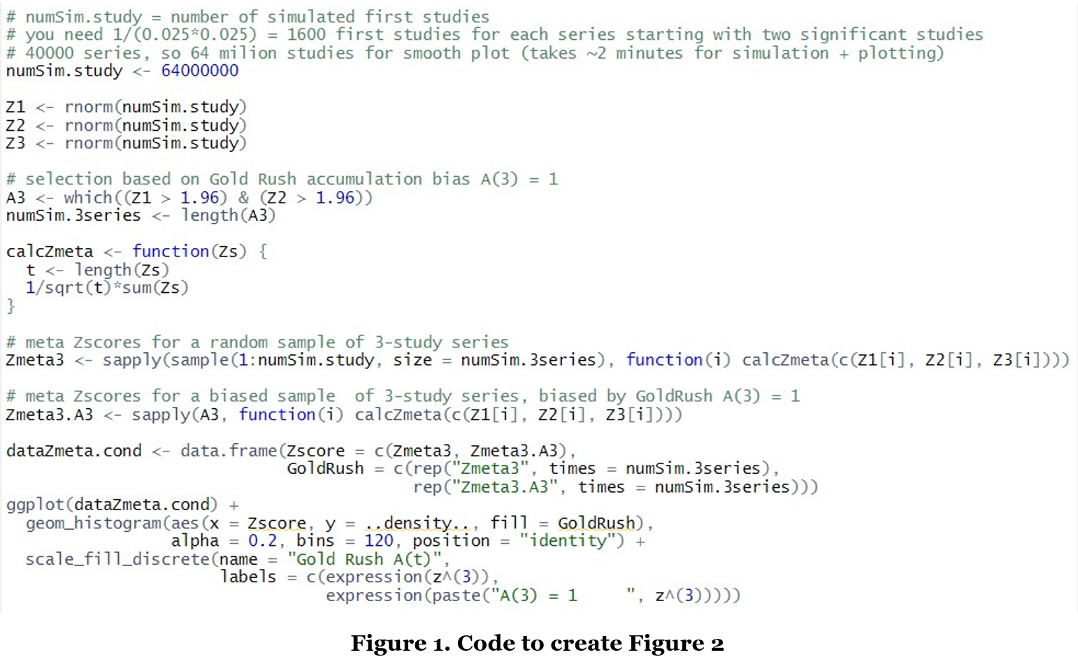
Theoretical sampling process: A fixed-effects meta-analysis assumes that if three studies z₁, z₂, z₃ are each sampled under the null hypothesis, each has a standard normal with mean zero and the standard normal sampling distribution also applies for the combined z⁽³⁾ score. The R code in Figure 1 illustrates this sampling process: First, a large population is simulated of possible first (Z1), second (Z2) and third (Z3) studies from a standard normal distribution. Then in Zmeta3 each index i represents a possible study series, such that c(Z1[i], Z2[i], Z3[i]) samples an unbiased study series and calcZmeta calculates its fixed-effects meta- analysis Z-score z⁽³⁾. So the large number of Z-scores in Zmeta3 capture the unbiased sampling distribution that is assumed for fixed-effects meta-analysis z⁽³⁾-scores.

Gold Rush sampling process: In contrast, the code resulting in A3 selects only those study series for which A(3) = 1 under extreme Gold Rush accumulation bias. So the large number of Z-scores in Zmeta3. A3 captures a biased sampling distribution for the fixed effects meta-analysis z⁽³⁾-scores.

Meta-analysis under Gold Rush accumulation bias: The final lines of code in Figure 1 plot two histograms of z⁽³⁾ samples, one with and one without the Gold Rush A(t) accumulation bias process, based on Zmeta3.A3 and Zmeta3 respectively. Figure 2 gives the result.

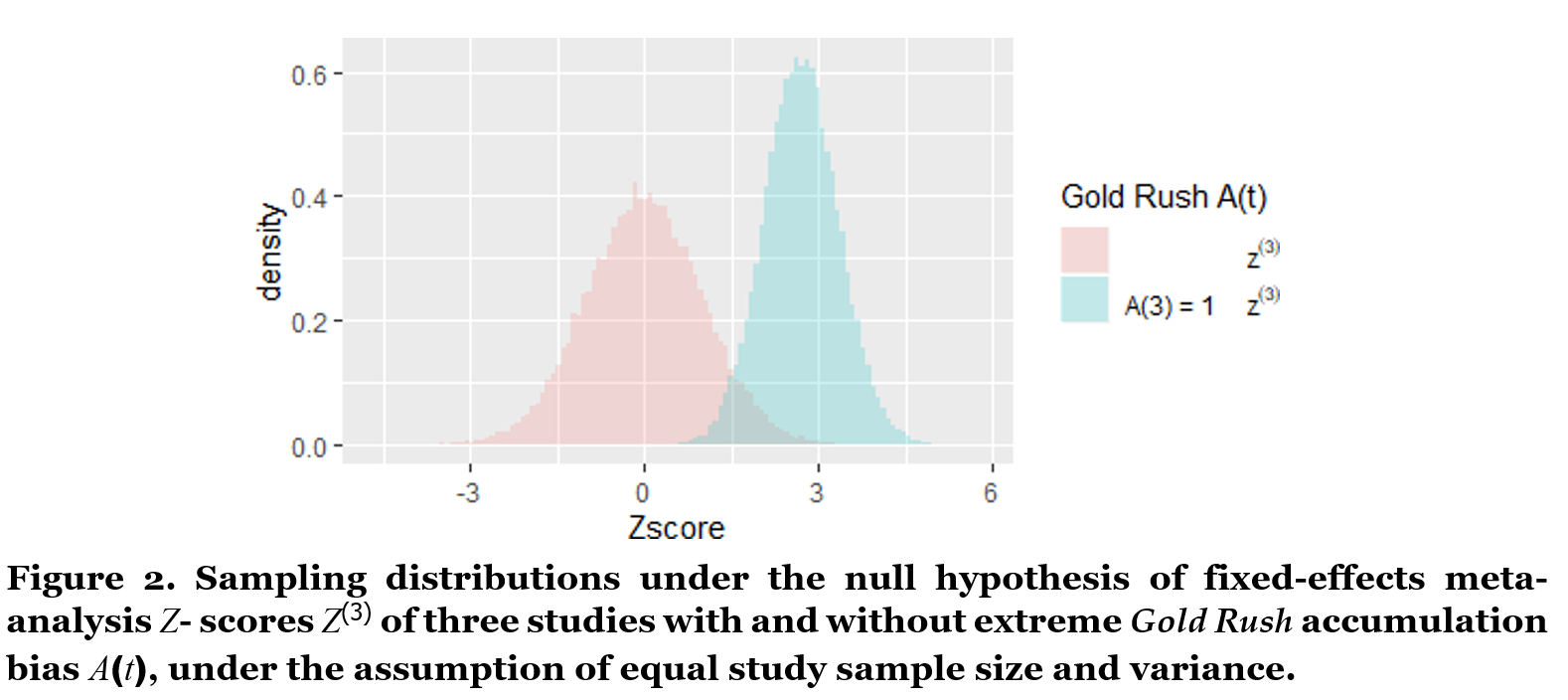
We observe in Figure 2 that the theoretical sampling process, resulting in the pink histogram, gives a distribution for the three-study meta-analysis z⁽³⁾-scores that is centered around zero. Under the Gold Rush sampling process, however, our three-study z⁽³⁾-scores do not behave like this theoretical distribution at all. The blue histogram has a smaller variance and is shifted to the right – representing the bias.

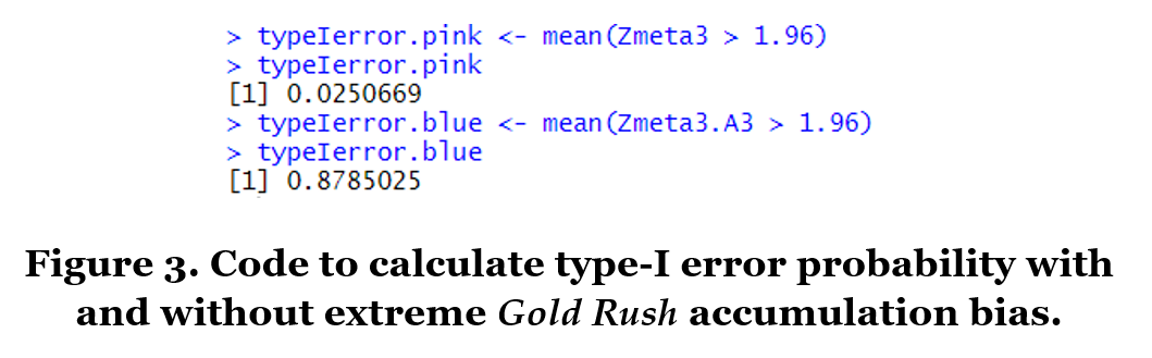
We conclude that we should not use conventional meta-analysis techniques to analyze our study series under Gold Rush accumulation bias: Conventional fixed-effects meta-analysis assumes that any three-study summary statistic Z⁽³⁾ is sampled from the pink distribution in Figure 2 under the null hypothesis, such that the meta- analysis is significant for Z⁽³⁾-scores larger than z_α = 1.96 for a right-sided test with type-I error control  α = 2.5%. Yet the actual blue sampling distribution under this accumulation bias process shows that a much larger fraction of series that accumulate three studies will have Z⁽³⁾-scores larger than 1.96 than is assumed by the theory of random sampling. This (extremely) inflated proportion of type-I errors is 88% instead of 2.5% in our extreme Gold Rush, and can be obtained from our simulation by the code in Figure 3.

Accumulation bias can be efficient

The steps in the code from Figure 1 that arrive at the biased distribution in Figure 2 illustrate that accumulation bias is in fact a selection bias. Nevertheless, accumulation bias does not result from questionable research practices, such as publication bias from file-drawering a selection of results. The selection to replicate only some studies instead of all of them biases the sampling distribution of study series, but can be a very efficient approach to set priorities in research and reduce research waste.

By inspecting our Gold Rush world a bit closer, we observe that a fixed-effects meta-analysis of three studies actually conditions on this number of studies ((A(t) needs to be A(3) to be 1), and that this conditional nature is what is driving the accumulation bias; in technical details subsection A.3 we show this explicitly. In the next section we take the unconditional view.

The unconditional sampling distribution under extreme Gold Rush accumulation bias

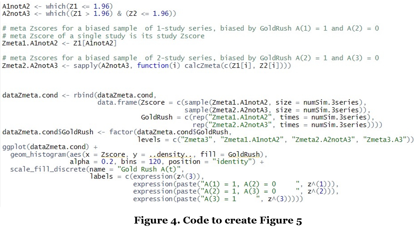
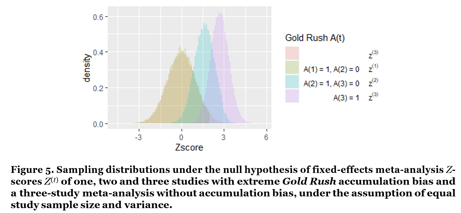
The R code in Figure 4 calculates the fixed-effects meta-analysis z⁽¹⁾, z⁽²⁾ and z⁽³⁾ scores, conditional on meta- analyzing a one-study, two-study, or three-study series in this adjusted Gold Rush accumulation bias scenario. The histograms of these conditional z^(t) scores are shown in Figure 5, including the theoretical unbiased z⁽³⁾ histogram that was also shown in Figure 2 and largely overlaps with the “A(1) = 1, A(2) = 0”-scenario. The difference between these two sampling distributions is only visible in their right tail, with the green histogram excluding values larger than z_α= 1.96 and redistributing their mass over other values.

Figure 5 clarifies that single studies are hardly biased in this extreme Gold Rush scenario, that the bias is problematic for two-study series and most extreme for three-study ones.

However, what this plot does not show us is how often we are in the one-study, two-study and three-study case.

To illustrate the relative frequencies of one-study, two-study and three-study meta-analyses, the code in Figure 6 samples the series in their respective numbers, instead of in equal numbers (which happens in the size = numSim.3series statement in Figure 4, part of creating the data frame). Plotting the total number of sampled Z-scores is dangerous for the single study z⁽¹⁾-scores, however, since there are so many of them (it can crash your R studio). So before plotting the histogram, a smaller sample (of size = 3*numSim.3series in total) is drawn that keeps the ratios between z⁽¹⁾s, z⁽²⁾s and z⁽³⁾s intact.

The histogram in Figure 7 illustrates an unconditional distribution by the raw counts of the z^(t)-scores: many result from a single study, very few from a two-study series and almost none from a three-study series. In fact, this unconditional sampling distribution is hardly biased, as we will illustrate with our table further below.

We first introduce an example of an ALL-IN meta-analysis to argue that such an unconditional approach can in fact be very efficient.

ALL-IN meta-analysis

Figure 8 shows an example of an ALL-IN meta-analysis. Each of the red/orange/yellow lines represents a study out of the ten separate studies in as many different countries. The blue line indicates the meta-analysis synthesis of the evidence; a live account of the evidence so far in the underlying studies. In fact, ALL-IN meta-analysis stands for Anytime, Live and Leading INterim meta-analysis, in which the Anytime Live property assures valid inference under continuously monitoring and the Leading property allows the meta-analysis results to inform whether individual studies should be stopped or expanded. This is important to note that such data-driven decisions would invalidate conventional meta-analysis by introducing accumulation bias.

To interpret Figure 8, we observe that initially only the Dutch (NL) study contributes to the meta-analysis and the blue line completely overlaps with the light yellow one. Very quickly, the Australian (AU) study also starts contributing and the blue meta-analysis line captures a synthesis of the evidence in two studies. Later on, also the study in the US, France (FR) and Uruguay (UY) start contributing and the meta-analysis becomes a three-study, four-study and five-study meta-analysis. How many studies contribute to the analysis, however, does not matter for its evidential value.

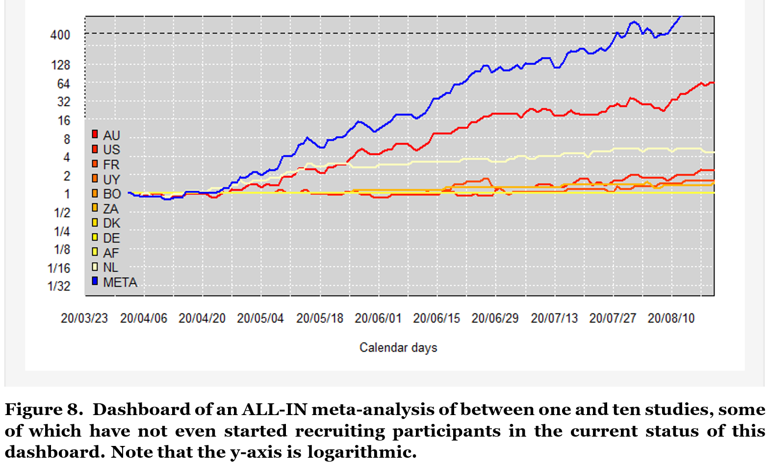
Some studies (like the Australian one) are much larger than others, such that under a lucky scenario this study could reach the evidential threshold even before other studies start observing data.  This threshold (indicated at 400) controls type-I errors at a rate of α= 1/400 = 0.0025 (details in the final section). So in repeated sampling under the null, the combined studies will only have a probability to cross this threshold that is smaller than 0.25%. In this repeated sampling the size of the study series is essentially random: we can be lucky and observe very convincing data in the early studies, making more studies superfluous, or we can be unlucky and in need of more studies. The threshold can be reached with a single study, with a two-study meta-analysis, with a three-study,.. etc, and the repeated sampling properties, like type-I error control, hold on average over all those sampling scenarios (so unconditional on the series size).

ALL-IN meta-analysis allows for meta-analyses with Type-I error control, while completely avoiding the effects of accumulation bias and multiple testing. This is possible for two reasons: (1) we do not just perform meta- analyses on study series that have reached a certain size, but continuously monitor study series irrespective of the current number of studies in the series; (2) we use likelihood ratios (and their cousins, e-values (Grünwald et al., 2019) instead of raw Z-scores and p-values; we say more on likelihood ratios further below.

Accumulation bias from ALL-IN meta-analysis vs Gold Rush

The ALL-IN meta-analysis in Figure 8 illustrates an improved efficiency by not setting the number of studies in advance, but let it rely on the data and be – just like the data itself – essentially random before the start of the research effort. This introduces dependencies between study results and series size that can be expressed in similar ways as Gold Rush accumulation bias. Yet this field of studies might make decisions differently to our Gold Rush: a positive nonsignificant result might not terminate the research effort, but encourage extra studies. And instead of always encouraging extra studies, a very convincing series of significant studies might conclude the research effort. If a series of studies is dependent on any such data-driven decisions, the use of conventional statistical methods is inappropriate. These dependencies actually do not have to be extreme at all: Many fields of research might be a bit like the Gold Rush scenario in their response to finding significant negative results of harm. A widely known study result that indicated significant harm might make it very unlikely that the series will continue to grow. So large study series will very rarely have a completely symmetric sampling distribution, since initial studies that observe results of significant harm do not grow into large series. Hence this small aspect of accumulation bias will already invalidate conventional meta-analysis, when it assumes such symmetric distributions under the null hypothesis with equal mass on significant effects of harm and benefit.

Properties averaged over time

Accumulation bias can already result from simply excluding results of significant harm from replication. This exclusion also takes place under extreme Gold Rush accumulation bias, since results of significant harm as well as all nonsignificant results are not replicated. Fortunately, any such scenarios can be handled by taking an unconditional approach to meta-analysis. We will now give an intuition for why this is true in case of our extreme Gold Rush scenario: initial studies have bias that balances the bias in larger study series when averaged over series size and analyzed in a certain way.

Table 1 is inspired by Senn (2014) (different question, similar answer) and represents our extreme Gold Rush world of study series.  It takes the same approach as Figure 7 and indicates the probability to meta-analyze   a one-study, two-study or three-study series of each possible form under the null hypothesis. The three study series are very biased, with two or even three out of three studies showing a positive significant effect. But the P₀ column shows that the probability of being in this scenario is very small under the null hypothesis, as was also apparent from Figure 7. In fact, most analysis will be of the one-study kind, that hardly have any bias, and are even slightly to the left of the theoretic standard null distribution. Exactly this phenomenon balances the biased samples of series of larger size.

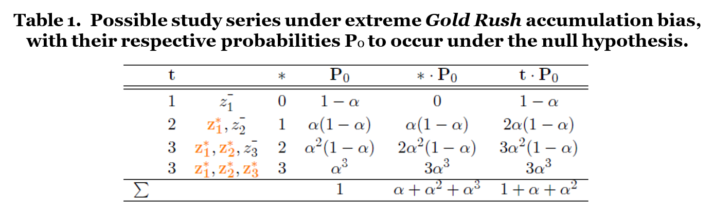
A Z-score is marked by a * and color orange (e.g.  z₁*)  in  case  the individual  study  result  is  significant  and  positive  (z₁ ≥ z_α  (one-sided test)) and  by  a (e.g.   z₁⁻)  otherwise.   The  column  t  indicates  the number of  studies  and  the  column counts the number of significant studies. The fifth and sixth column multiply P₀ with the column and t column to arrive at an expected value E0[*] and E0[t] respectively in the bottom row.

The bottom row of Table 1 gives the expected values for the number of significant studies per series in the *P₀ column, and the expected value for the total number of studies per series in the t P₀ column. If we use these expressions to obtain the proportion of expected number of significant to expected total number of studies, we get the following:

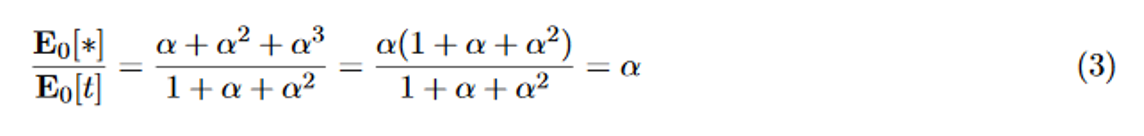
The proportion of expected significant effects to expected series size is still α in Table 1 under extreme Gold Rush accumulation bias, as it would also be without accumulation bias.

This result is driven by the fact that there is a martingale process underlying this table. If a statistic is a martingale process and it has a certain value after t studies, the conditional expected value of the statistic after t + 1 studies, given all the past data, is equal to the statistic after t studies. So if our proportion of significant positive studies is exactly α for the first study (t = 1),  we  expect to also observe a proportion α if we  grow  our series with an additional study (t = 1+1 = 2). The Accumulation bias does not affect such statistics when averaged over time if martingales are involved (Doob’s optional stopping theorem for martingales). You can verify this aspect by deleting the last row for z₁*, z₂*, z₃*  from our table and adding two rows for t = 4 in its place with z₁*, z₂*, z₃*   and either a fourth significant or a nonsignificant study.  If you calculate the expected significant effects to expected series size, you will again arrive at α.

Martingale properties drive many approaches to sequential analysis, including the Sequential Probability Ratio Test (SPRT), group-sequential analysis and alpha spending. When applied to meta-analysis, any such inferences essentially average over series size, just like ALL-IN meta-analysis.

Multiple testing over time

Just having the expectation of some statistics not affected by stopping rules is not enough to monitor data continuously, as in ALL-IN meta-analysis. We need to account for the multiple testing as well. In that respect, the approaches to sequential analysis differ by either restricting inference to a strict stopping rule (SPRT), or setting a maximum sample size (group-sequential analysis and alpha spending).

ALL-IN meta-analysis takes an approach that is different from its predecessors and is part of an upcoming field of sequential analysis for continuous monitoring with an unlimited horizon. These approaches are called Safe for optional stopping and/or continuation (Grünwald et al., 2019) any-time valid (Ramdas et al., 2020). Their methods rely on nonnegative martingales (Ramdas et al., 2020); with its most well-known and useful martingale: the likelihood ratio. For a meta-analysis Z-score, a martingale process of likelihood ratios could look as follows:

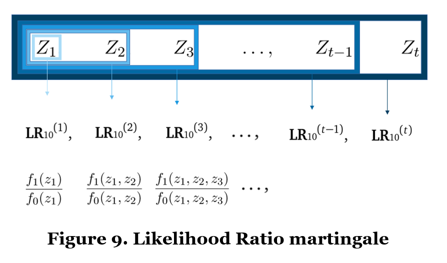
The subscript ₁₀ indicates that the denominator of the likelihood ratio is the likelihood of the Z-scores under the null hypothesis of mean zero, and in the numerator is some alternative mean normal likelihood. The likelihood ratio becomes smaller when the data are more likely under the null hypothesis, but the likelihood ratio can never become smaller than 0 (hence the “nonnegative” martingale). This is crucial, because a nonnegative martingale allows us to use Ville’s inequality (Ville, 1939), also called the universal bound by Royall (1997). For likelihood ratios, this means that we can set a threshold that guarantees type-I error control under any accumulation bias process and at any time, as follows:

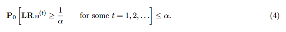
The ALL-IN meta-analysis in Figure 8 in fact is based on likelihood ratios like this, and controls the type-I error by the threshold 400 at level 1/400 = 0.25%.

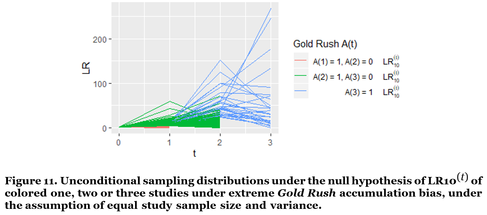
The code below illustrates that likelihood ratios can also control type-I error rates under continuous monitoring when extreme Gold Rush accumulation bias is at play. Within our previous simulation, we again assume a Gold Rush world with only true null studies and very biased two-study and three-study series. The code in Figure 11 calculates likelihood ratios for the growing study series under accumulation bias. Figure 11 illustrates that still very few likelihood ratios ever grow very large.

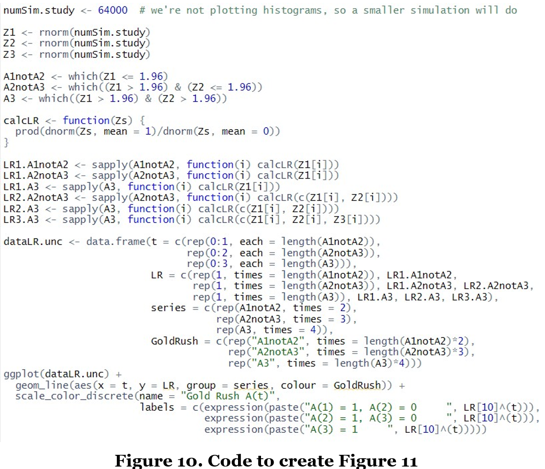
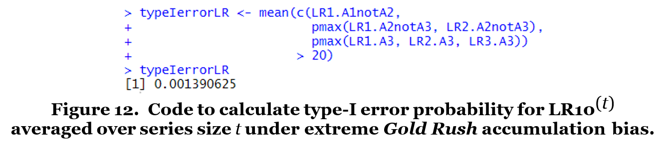
If we set our type-I error rate α to 5%, and compare our likelihood ratios to 1/α = 20 we observe that less than  1/20 = 5% of  the  study  series  ever achieves  a  value  of  LR₁₀   larger  than  20 (Figure 12).  The  simulated type-I error is even much smaller than 5% since in our Gold Rush world series stop growing at three studies, yet this procedure controls type-I error also in the case none of these series stops growing at three studies, but all continue to grow forever.

The type-I error control is thus conservative, and we pay a small price in terms of power. That price is quite manageable, however, and can be tuned by setting the mean value of the alternative likelihood (arbitrarily set to mean = 1 in the code for calcLR of Figure 10). More on that in Grünwald et al. (2019) and the forthcoming preprint paper on ALL-IN meta-analysis that will appear on https://projects.cwi.nl/safestats/.

It is this small conservatism in controlling type-I error that allows for full flexibility: There isn’t a single accumulation bias process that could invalidate the inference. Any data-driven decision is allowed. And data- driven decisions can increase the value of new studies and reduce research waste.

Conclusion

In our imaginary world of extreme Gold Rush accumulation bias, the sampling distribution of the meta-analysis Z-score behaves very different from the sampling distribution assumed to calculate p-values and confidence intervals. A meta-analysis p-value conditions on the available sample size – on the sample size of the studies and on the number of studies available – and represents the tail area of this conditional sampling distribution under the null based on the observed Z-statistic. Analogously, a meta-analysis confidence interval provides coverage under repeated sampling from this conditional distribution. So if this sample size is driven by the data, as in any accumulation bias process, there is a mismatch between the assumed sampling distribution of the meta-analysis Z-statistic, and the actual sampling distribution.

We believe that some accumulation bias is at play in almost any retrospective meta-analysis, such that p-values and confidence intervals generally do not have their promised type-I error control and coverage. ALL-IN meta- analysis based on likelihood ratios can handle accumulation bias, even if the exact process is unknown. It also allows for continuous monitoring; multiple testing is no problem. Hence taking the ALL-IN perspective on meta-analysis will reduce research waste by allowing efficient data-driven decisions – not letting them invalidate the inference – and incorporating single studies and small study series into meta-analysis inference.

Postscript

ALL-IN meta-analysis has been applied during the corona pandemic to analyze an accumulating series of studies while they were still ongoing. Each study investigated the ability of the BCG vaccine to prevent covid-19, but data on covid cases came in only slowly (fortunately). Meta-analyzing interim results and data-driven decisions improved the possibility of finding efficacy earlier in the pandemic. A webinar on the methodology underlying this meta-analysis – the specific likelihood ratios – is available on https://projects.cwi.nl/safestats/ under the name ALL-IN-META-BCG-CORONA.

Judith ter Schure is a PhD student in the Department of Machine Learning at Centrum Wiskunde & Informatica in the Netherlands. She can be contacted at Judith.ter.Schure@cwi.nl.

Acknowledgements

My thanks go to Professor Bob Reed for inviting this contribution to his website and his patience with its publication. I also want to acknowledge Professor Peter Grünwald for checking the details. Daniel Lakens provided me with great advice to write this text more blog-like. Muriel Pérez helped me with the details of the martingale underlying the table.

References

Iain Chalmers and Paul Glasziou. Avoidable waste in the production and reporting of research evidence. The Lancet, 114(6):1341–1345, 2009.

Iain Chalmers, Michael B Bracken, Ben Djulbegovic, Silvio Garattini, Jonathan Grant, A Metin Gülmezoglu, David W Howells, John PA Ioannidis, and Sandy Oliver. How to increase value and reduce waste when research priorities are set. The Lancet, 383(9912):156–165, 2014.

Hans Lund, Klara Brunnhuber, Carsten Juhl, Karen Robinson, Marlies Leenaars, Bertil F Dorch, Gro Jamtvedt, Monica W Nortvedt, Robin Christensen, and Iain Chalmers. Towards evidence based research. Bmj, 355: i5440, 2016.

Judith ter Schure and Peter Grünwald. Accumulation Bias in meta-analysis: the need to consider time in error control [version 1; peer review: 2 approved]. F1000Research, 8:962, June 2019. ISSN 2046-1402. doi: 10.12688/f1000research.19375.1. URL https://f1000research.com/articles/8-962/v1.

Steven P Ellis and Jonathan W Stewart. Temporal dependence and bias in meta-analysis. Communications in Statistics—Theory and Methods, 38(15):2453–2462, 2009.

Elena Kulinskaya, Richard Huggins, and Samson Henry Dogo. Sequential biases in accumulating evidence. Research synthesis methods, 7(3):294–305, 2016.

Peter Grünwald, Rianne de Heide, and Wouter Koolen. Safe testing. arXiv preprint arXiv:1906.07801, 2019.

Stephen Senn. A note regarding meta-analysis of sequential trials with stopping for efficacy. Pharmaceutical Statistics, 13(6):371–375, 2014.

Aaditya Ramdas, Johannes Ruf, Martin Larsson, and Wouter Koolen. Admissible anytime-valid sequential inference must rely on nonnegative martingales. arXiv preprint arXiv:2009.03167, 2020.

Jean Ville. Etude critique de la notion de collectif. Bull. Amer. Math. Soc, 45(11):824, 1939.

Richard Royall. Statistical evidence: a likelihood paradigm, volume 71. CRC press, 1997.

Judith ter Schure, Alexander Ly, Muriel F. Pérez-Ortiz, and Peter Grünwald. Safestats and all-in meta-analysis project page. https://projects.cwi.nl/safestats/, 2020.

This blog post discusses approaches to meta-analysis that control type-I error averaged over study series size. This is called error control surviving over time in Ter Schure and Grünwald (2019), as will become more clear in the technical details.

The R code used in this blog and a pdf with technical details can be found here.