[* EiR = Econometrics in Replications, a feature of TRN that highlights useful econometrics procedures for re-analysing existing research.]

NOTE: This blog uses Stata for its estimation. All the data and code necessary to reproduce the results in the tables below are available at Harvard’s Dataverse: click here.

Missing data is ubiquitous in economics. Standard practice is to drop observations for which any variables have missing values. At best, this can result in diminished power to identify effects. At worst, it can generate biased estimates. Old-fashioned ways to address missing data assigned values using some form of interpolation or imputation. For example, time series data might fill in gaps in the record using linear interpolation. Cross-sectional data might use regression to replace missing values with their predicted values. These procedures are now known to be flawed (Allison, 2001; Enders, 2010).

The preferred way to deal with missing data is to use maximum likelihood (ML) or multiple imputation (MI), assuming the data are “missing at random”. Missing at random (MAR) essentially means that the probability a variable is missing is independent of the value of that variable. For example, if a question about illicit drug use is more likely to go unanswered for respondents who use drugs, then those data would not be MAR. Assuming that the data are MAR, both ML and MI will produce estimates that are consistent and asymptotically efficient.

ML is in principle the easiest to perform. In Stata, one can use the structural equation modelling command (“sem”) with the option “method(mlmv)”. That’s it! Unfortunately, the simplicity of ML is also its biggest disadvantage. For linear models, ML simultaneously estimates means, variances, and covariances while also accounting for the incomplete records associated with missing data. Not infrequently, this causes convergence problems. This is particularly a problem for panel data where one might have a large number of fixed effects.

In this blog, we illustrate how to apply both ML and MI to a well-cited study on mortality and inequality by Andrew Leigh and Christopher Jencks (Journal of Health Economics, 2007). Their analysis focused on the relationship between life expectancy and income inequality, measured by the share of pre-tax income going to the richest 10% of the population. Their data consisted of annual observations from 1960-2004 for Australia, Canada, France, Germany, Ireland, the Netherlands, New Zealand, Spain, Sweden, Switzerland, the UK, and the US. We use their study both because their data and code are publicly available, and because much of the original data were missing.

The problem is highlighted in TABLE 1, which uses a reconstruction of L&J’s original dataset. The full dataset has 540 observations. The dependent variable, “Life expectancy”, has approximately 11 percent missing values. The focal variable, “Income share of the richest 10%”, has approximately 24 percent missing values. The remaining control variables vary widely in their missingness. Real GDP has no missing values. Education has the most missing values, with fully 80% of the variable’s values missing. This is driven by the fact that the Barro and Lee data used to measure education only reports values at five-year intervals.

In fact, the problem is more serious than TABLE 1 indicates. If we run the regression using L&J’s specification (cf. Column 7, Table 4 in their study), we obtain the results in Column (1) of TABLE 2. The estimates indicate that a one-percentage point increase in the income share of the richest 10% is associated with an increase in life expectancy of 0.003 years, a negligible effect in terms of economic significance, and statistically insignificant. Notably, this estimate is based on a mere 64 observations (out of 540).

In fact, these are not the results that L&J reported in their study. No doubt because of the small number of observations, they used linear interpolation on some (but not all) of their data to fill in missing values. Applying their approach to our data yields the results in Column (2) of Table 2 below. There are two problems with using their approach.

First, for various reasons, L&J did not fill in values for all the missing values. The ended up using only 430 out of a possible 540 observations. As a result, their estimates did not exploit all the information that was available to them. Second, interpolation replaces missing values with their predicted values without accounting for the randomness that occurs in real data. This biases standard errors, usually downwards. ML and MI allow one to do better.

ML is the easiest method to apply. To estimate the regression in Table 2 requires a one-line command:

sem (le <- ts10 gdp gdpsq edu phealth thealth id2-id12 year2-year45), method(mlmv) vce(cluster id)

The “sem” command calls up Stata’s structural equation modelling procedure. The option “method(mlmv)” tells Stata to use maximum likelihood to accommodate missing values. If this option is omitted from the above, then the command will produce results identical to those in Column 1 of Table 1, except that the standard errors will be slightly smaller.

While the simplicity of ML is a big advantage, it also introduces complications. Specifically, ML estimates all the parameters simultaneously. The inclusion of 11 country fixed effects and 44 year dummies makes the number of elements in the variance-covariance matrix huge. This, in combination with the fact that ML simultaneously integrates over distributions of variables to account for missing values creates computational challenges. The ML procedure called up by the command above did not converge after 12 hours. As a result, we next turn to MI.

Unlike ML, MI fills in missing values with actual data. The imputed values are created to incorporate the randomness that occurs in real data. The most common MI procedure assumes that all of the variables are distributed multivariate normal. It turns out that this is a serviceable assumption even if the regression specification includes variables that are not normally distributed, like dummy variables (Horton et al., 2003; Allison, 2006).

As the name suggests, MI creates multiple datasets using a process of Monte Carlo simulation. Each of the datasets produces a separate set of estimates. These are then combined to produce one overall set of estimation results. Because each data set is created via a simulation process that depends on randomness, each dataset will be different. Furthermore, unless a random seed is set, different attempts will produce different results. This is one disadvantage of MI versus ML.

A second disadvantage is that MI requires a number of subjective assessments to set key parameters. The key parameters are (i) the “burnin”, the number of datasets that are initially discarded in the simulation process; (ii) the “burnbetween”, the number of intervening datasets that are discarded between retained datasets to maintain dataset independence; and (iii) the total number of imputed datasets that are used for analysis.

The first two parameters are related to the properties of “stationarity” and “independence”. The analogue to convergence in estimated parameters in ML is convergence in distributions in MI. To assess these two properties we first do a trial run of imputations.

The command “mi impute mvn” identifies the variables with missing values to the left of the “=” sign, while the variables to the right are identified as being complete.

mi impute mvn le ts10 edu phealth thealth im  = gdp gdpsq id2-id12 year2-year45, prior(jeffreys)  mcmconly rseed(123) savewlf(wlf, replace)

The option “mcmconly” lets Stata know that we are not retaining the datasets for subsequent analysis, but only using them to assess their characteristics.

The option “rseed(123)” ensures that we will obtain the same data every time we run this command.

The option “prior(jeffreys)” sets the posterior prediction distribution used to generate the imputed datasets as “noninformative”. This makes the distribution used to impute the missing values solely determined by the estimates from the last regression. 

Lastly, the option “savewlf(wlf, replace)” creates an aggregate variable called the “worst linear function” that allows one to investigate whether the imputed datasets are stationary and independent.

Note that Stata sets the default values for “burnin” and “burnbetween” at 100 and 100.

The next set of key commands are given below.

use wlf, clear

tsset iter

tsline wlf, ytitle(Worst linear function) xtitle(Burn-in period) name(stable2,replace)

ac wlf, title(Worst linear function) ytitle(Autocorrelations) note(“”) name(ac2,replace)

The “tsline” command produces a “time series” graph of the “worst linear function” where “time” is measured by number of simulated datasets. We are looking for trends in the data. That is, do the estimated parameters (which includes elements in the variance-covariance matrix) tend to systematically depart from the overall mean.

The graph above is somewhat concerning because it appears to first trend up and then trend down. As a result, we increase the “burnin” value to 500 from its default value of 100 with the following command. Why 500? We somewhat arbitrarily choose a number that is substantially larger than the previous “burnin” value.

mi impute mvn le ts10 edu phealth thealth im  = gdp gdpsq id2-id12 year2-year45, prior(jeffreys) mcmconly burnin(500) rseed(123) savewlf(wlf, replace)

…

use wlf, clear

tsset iter

tsline wlf, ytitle(Worst linear function) xtitle(Burn-in period) name(stable2,replace)

ac wlf, title(Worst linear function) ytitle(Autocorrelations) note(“”) name(ac2,replace)

This looks a lot better. The trending that is apparent in the first half of the graph is greatly reduced in the second half. We subjectively determine that this demonstrates sufficient “stationarity” to proceed. Note that there is no formal test to determine stationarity.

The next thing is to check for independence. The posterior distributions used to impute the missing values rely on Bayesian updating. While our use of the Jeffrys prior reduces the degree to which contiguous imputed datasets are related, there is still the opportunity for correlations across datasets. The “ac” command produces a correlogram of the “worst linear function” that allows us to assess independence. This is produced below.

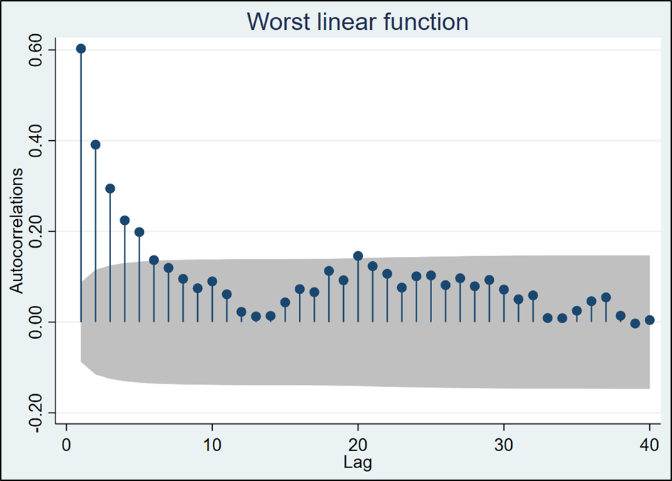
This correlogram indicates that as long as we retain imputed datasets that are at least “10 datasets apart”, we should be fine. The default value of 100 for “burnbetween” is thus more than sufficient.

The remaining parameter to be set is the total number of imputed datasets to use for analysis. For this we use a handy, user-written Stata (and SAS) command from von Hippel (2020) called “how_many_imputations”.

The problem with random data is that it produces different results each time. “how_many_imputations” allows us to set the number of imputations so that the variation in estimates will remain within some pre-determined threshold value. The default value is to set the number of imputations so that the coefficient of variation of the standard error of the “worst linear function” is equal to 5%.

It works like this. First we create a small initial set of imputed datasets. The command below imputes 10 datasets (“add(10)”).

mi impute mvn le ts10 edu phealth thealth im  = gdp gdpsq id2-id12 year2-year45, prior(jeffreys) burnin(500) add(10) rseed(123)

We then estimate a fixed effects regression for each of the 10 datasets. Note that we use the standard Stata command for “xtreg, fe” after “mi estimate:”

mi xtset id year

mi estimate: xtreg le ts10 gdp gdpsq edu phealth thealth year2-year45, fe vce(cluster id)

how_many_imputations

The command “how_many_imputations” determines the number of imputed datasets calculated to produce standard errors with a coefficient of variation for the standard errors equal to 5%. In this particular case, the output is given by:

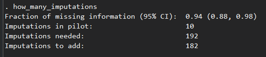
The output says to create 182 more imputed datasets.

We can feed this number directly into the “mi impute” command using the “add(`r(add_M)’)” option:

mi impute mvn le ts10 edu phealth thealth im  = gdp gdpsq id2-id12 year2-year45, prior(jeffreys) burnin(500) add(`r(add_M)’)

After running the command above, our stored data now consists of 104,220 observations: The initial set of 540 observations plus 192 imputed datasets × 540 observations/dataset. To combine the individual estimates from each dataset to get an overall estimate, we use the following command:

mi xtset id year

mi estimate: xtreg le ts10 gdp gdpsq edu phealth thealth year2-year45, fe vce(cluster id)

The results are reported in Column (3) of Table 2. A further check re-runs the program using different seed numbers. These show little variation, confirming the robustness of the results.

In calculating standard errors, Table 2 follows L&J’s original procedure of estimating standard errors clustered on countries. One might want to improve on this given that their sample only included 12 countries.

An alternative to the “mi estimate” command above is to use a user-written program that does wild cluster bootstrapping. One such package is “wcbregress”.  While not all user-written programs can be accommodated by Stata’s “mi estimate”, one can use wcb by modifying the “mi estimate” command as follows:

mi estimate, cmdok: wcbregress le ts10 gdp gdpsq edu phealth thealth year2-year45, group(id)

A comparison of Columns (3) and (1) reveals what we have to show for all our work. Increasing the number of observations substantially reduced the sizes of the standard errors. The standard error of the focal variable, “Income share of the richest 10%”, decreased from 0.051 to 0.035.

While the estimated coefficient remained statistically insignificant for this variable, the smaller standard errors boosted two other variables into significance: “Real GDP per capital squared” and “Log public health spending pc”. Furthermore, the larger sample provides greater confidence that the estimated coefficients are representative of the population from which we are sampling.

Overall, the results provide further support for Leigh & Jencks (2007)’s claim that the relationship between inequality and mortality is small and statistically insignificant.

Given that ML and MI estimation procedures are now widely available in standard statistical packages, they should be part of the replicator’s standard toolkit for robustness checking of previously published research. 

Weilun (Allen) Wu is a PhD student in economics at the University of Canterbury. This blog covers some of the material that he has researched for his thesis. Bob Reed is Professor of Economics and the Director of UCMeta at the University of Canterbury. They can be contacted at weilun.wu@pg.canterbury.ac.nz and bob.reed@canterbury.ac.nz, respectively.

REFERENCES

Allison, P. D. (2001). Missing data. Sage publications.

Enders, C. K. (2010). Applied missing data analysis. Guilford press.

Leigh, A., & Jencks, C. (2007). Inequality and mortality: Long-run evidence from a panel of countries. Journal of Health Economics, 26(1), 1-24.

Horton, N. J., Lipsitz, S. R., & Parzen, M. (2003). A potential for bias when rounding in multiple imputation. The American Statistician, 57(4), 229-232.

Allison, P. (2006, August). Multiple imputation of categorical variables under the multivariate normal model. In Annual Meeting of the American Sociological Association, Montreal.

Von Hippel, P. T. (2020). How many imputations do you need? A two-stage calculation using a quadratic rule. Sociological Methods & Research, 49(3), 699-718.