REED: EiR* – Heterogeneity in Two-Way Fixed Effects Models
[* EiR = Econometrics in Replications, a feature of TRN that highlights useful econometrics procedures for re-analysing existing research. The material for this blog is drawn from the recent working paper “Two-way fixed effects estimators with heterogeneous treatment effects” by Clément de Chaisemartin and Xavier D’Haultfoeuille, posted at ArXiv.org]
NOTE #1: All the data and code (Stata) necessary to produce the results in the tables below are available at Harvard’s Dataverse: click here.
NOTE #2: Since this blog was written, the “breps” and “brepscluster” options have been removed from the twowayfeweights command (see below).
It is common to estimate treatment effects within a model incorporating both group and time fixed effects (think Differences-in-Differences). In a recent paper, Clément de Chaisemartin and Xavier D’Haultfoeuille (henceforth C&D) demonstrate how these models can produce unreliable estimates of average treatment effects when effects are heterogeneous across groups and time periods.
Their paper both identifies the problem and provides a solution. The purpose of this blog is to enable others to use C&D’s procedures to re-analyze published research.
In what follows, I highlight key points from their paper. Following their paper, I illustrate the problem, discuss the solution, and show how it makes a difference in replicating a key result from Gentzkow et al. (2011).
The Problem
Consider the following two-group, three-period data, where groups are designated by g = 0,1 and time periods by t = 0,1,2.
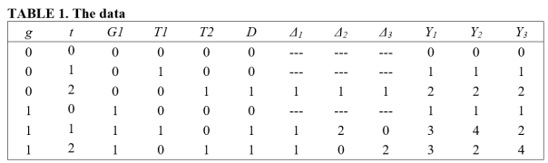
G1, T1, and T2 are dummy variables indicating whether an observation belongs to the first group, first time period, and second time period, respectively. D is a treatment indicator that takes the value 1 if the particular (g,t) cell received treatment. Note that treatment is applied to group g=0 at time t=2, and to group g=1 at times t=1,2.
Δ indicates the size of the treatment effect for treated cells (we ignore the size of the treatment effect for the untreated cells). Consider three regimes for Δ.
In the first regime (Δ1), the treatment effect is homogeneous across groups and time periods. In the second regime (Δ2), the treatment effects are heterogeneous, with the treatment effect equalling 1 for (g,t) = (0,2), and 2 and 0 for cells (g,t) = (1,1) and (g,t) = (1,2), respectively. The third regime (Δ3) is similar, except that the sizes of the treatment effects are reversed for group g=1, with treatment effects equal to 0 and 2 in time periods 1 and 2. Note that the average treatment effect for the treated (ATT) equals 1 for all three treatment regimes.
Let the outcome for each observation be determined by the following equation:
Ygt = Δgt∙Dgt + G1gt + T1gt + T2gt , g=0,1; t=0,1,2.
Suppose one estimates the following regression specification using OLS:
(1) Ygt = β0 + βfe Dgt + βG1G1gt + βT1T1gt + βT2T2gt + error.
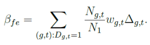
In this specification, the treatment effect is estimated by βfe, the coefficient on the treatment dummy variable. C&D prove that βfe can be expressed as a weighted average of the individual treatment effects:
βfe = w02Δ02 + w11Δ11 + w12Δ12 ,
where w02 + w11 + w12 = 1; and Δ02 , Δ11, and Δ12 represent the treatment effects associated with the (g,t) cells (0,2), (1,2), and (1,3) for a given treatment regime.
What follows is quite surprising. C&D demonstrate that the weights need not all be positive. In fact, it can be shown in the current case that:
βfe = (½ Δ02) + Δ11 + (-½ Δ12) .
Where does the negative weight on the third treatment effect come from? βfe is the average of two difference-in-differences. The first is associated with the change in treatment for g=0 over the time periods t=1,2 (DID0). The second relates to the change in treatment for g=1 over the time periods t=0,1 (DID1). Specifically,
βfe = (DID0 + DID1)/2.
First consider DID0 = [E(Y02) – E(Y01)] -[E(Y12) – E(Y11)] = Δ02 – (Δ12 – Δ11).
The first term in brackets in DID0 measures the change in outcomes for the treatment observations associated with the first change in treatment. The second term in brackets represents the change in outcomes for the control observations over the same period. Note that both control observations receive treatment.
Ignoring time trends (as they cancel out under the common trend assumption), if treatment effects are homogeneous, the latter term, [E(Y12) – E(Y11)] = (Δ12 – Δ11), will drop out. But if the treatment effect for group g=1 is different for periods t=1,2, this term remains. Further, if the treatment effect in t=2 is sufficiently large relative to t=1, this will dominate Δ02, and DID0 will be negative.
Next consider DID1 = [E(Y11) – E(Y10)] -[E(Y01) – E(Y00)] = Δ11.
In this case, heterogeneity in treatment effects is not an issue because the control observations, represented by the last term in brackets, consist of two untreated observations.
What is important to note here is that βfe = (DID0 + DID1)/2 can be negative even if all the individual treatment effects are positive!
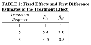
The table below reports the values for βfe for each of the three treatment regimes (Δ1, Δ2, Δ3). Also reported are the values of the first difference estimator, βfd, which, in this case of two groups and three time periods, is equal to the fixed effects estimator. (Note that in general, βfe ≠ βfd, a fact that we will exploit below.)
Of particular interest is the third treatment regime, where βfe = βfd < 0, even though all the individual treatment effects (Δ02 , Δ11, and Δ12) are greater than zero.
The case above demonstrates how heterogeneity can cause estimates of the average treatment effect to be negative even though the individual treatment effects are all positive. More generally, βfe will not be the same as βfd; and given heterogeneity, either one, or the other, or both can be a biased estimate of the average treatment effect on the treated (ATT).
How Do You Know If You Have a Problem?
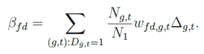
Define ΔTR as the ATT, weighted by the number of individuals in each (g,t) cell:
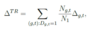
(in the example above, Ngt = 1 and N1 = 3).
βfe and βfd are also weighted measures of the ATT, but they have an additional set of weights (wgt and wfd,gt, respectively).
Note that βfe and βfd employ different weights wg,t and wfd,g,t. A necessary condition for both estimators to provide an unbiased estimate of ΔTR is that the weighting terms wg,t and wfd,g,t be uncorrelated with the respective treatment effects.
Thus, one diagnostic is to test for a significant difference between βfe and βfd.. If the two estimates are significantly different, that is an indicator that at least one of the two estimators is a biased estimator of the overall treatment effect.
Another diagnostic is to regress the weights on a variable that is associated with the size of the treatment effect. If one finds a significant correlation, then that is an indicator that the respective estimator (βfe or βfd.) is a biased estimator of ΔTR.
The Solution
C&D propose an estimator that focuses on treatment changes. The estimator compares treatment changes over consecutive time periods (either untreated or treated, or treated to untreated) with other observations during the same time period whose treatment did not change. They call this estimator the WTC estimator, for Wald-Time Corrected. While the example above consisted of a very restricted case (binary treatment, only one observation per (g,t) cell), their estimator generalizes to cases where treatment is continuous, and where only a portion of individuals in a given (g,t) cell receive treatment.
As a check on their estimator, they suggest a placebo estimator. The placebo estimator relates treatment changes to outcomes from the preceding period. Under the “common trends” assumption, the placebo estimator WplTC should equal zero. Failure to reject this hypothesis provides some evidence that the assumptions underlying the WTC estimator are valid.
A Replication Application
In their paper, C&D replicate results from the study, “The Effect of Newspaper Entry and Exit on Electoral Politics”, published in the American Economic Review in 2011 by Matthew Gentzkow, Jesse Shapiro, and Michael Sinkinson (GSS). GSS use county-level data from the US for the years 1868-1928 to estimate the relationship between Presidential turnout and the number of newspapers in a county. Following C&D, I explain how to implement their procedures and compare their results with those reported by GSS.
In the notation of the leading example above,
Ygt = Presidential turnout in county g at time t,
Dgt = Number of newspapers in county g at time t.
GSS use a first-difference estimator to estimate the effect of an additional newspaper on Presidential turnout. Their difference specification includes state-year fixed effects, and clusters on counties. They estimate that an additional newspaper in a county increased Presidential turnout by 0.26 percentage points (average Presidential turnout was approximately 65 percent during this period). Their estimate is reported below (cf. βfd). C&D use GSS’s data to also estimate a conventional fixed effects estimate and this is also reported in the table (cf. βfe). Note that the fixed effects estimator produces a negative estimate.

C&D first test H0: βfd = βfe and obtain a t-stat of 2.86, rejecting the null at conventional levels of significance. This indicates that at least one of these is a biased estimator of the overall treatment effect.
As a further test, C&D estimate the relationship between the respective weights, wfd,gt and wgt, and the treatment effect. Of course, the treatment effect is unobserved. As a proxy for the size of the treatment effect, C&D use year. C&D hypothesize that the effect of newspapers might change over time as other sources of communication, such as radio towards the end of the period, became more important.
To estimate this relationship, C&D employ a user-written Stata program called twowayfeweights. An example command for βfe is given below.
twowayfeweights prestout cnty90 year numdailies, type(feTR) controls(styr1-styr666) breps(100) brepscluster(cnty90) test_random_weights(year)
The command is twowayfeweights. The outcome variable is presidential turnout (prestout), the group and time variables are cnty90 and year, respectively. The treatment variable is numdailies. The option type identifies whether one is estimating weights for βfe or βfd (the syntax for βfd is slightly different). controls and breps identify, respectively, the other variables in the equation (here, state and year fixed effects), and the number of bootstrap replications to run. brepscluster indicates that the bootstrapping should be blocked according to county. The last option, test_random_weights regresses the respective weights on the variable assumed to be related to the size of the treatment effect (year). Note that while the weights are not automatically saved, there is an option to save them so that one can observe how they vary across counties and years. The results are reported below.

The results suggest that βfd may be adversely affected by correlation between the weights and the treatment effect, causing it to be a biased estimator of the overall average treatment effect on the treated. Note, however, that the sign of the correlation does not, per se, indicate the sign of the associated bias. On the other hand, the fixed effects estimator does not demonstrate evidence that the corresponding weights are correlated with treatment effects.
The last step consists of estimating the treatment effect using the WTC estimator. To do that, we use another user-written Stata program called fuzzydid:
fuzzydid prestout G_T G_T_for year numdailies, tc newcateg(0 1 2 1000) qualitative(st1-st48)
The syntax is similar to twowayfeweights, except that following the outcome variable (prestout) are two indicator variables. These indicate whether the treatment variable (numdailies) increased (G_T=1), decreased (G_T=-1) or stayed the same (G_T=0), compared to the preceding election period. G_T_for is the lead value of G_T in the immediately succeeding election period.
The options indicate that the Wald-Time Corrected statistic is to be calculated (tc), newcateg lumps the number of newspapers into 4 categories (0, 1, 2, and >2), and that state fixed effects should be included in the estimation (qualitative).
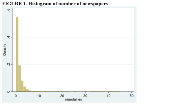
The reason for combining numbers of newspapers greater than 2 into a single category is that control groups need to have the same number of “treatments” as the treatment group. From the histogram below, it is apparent that relatively few counties have more than two newspapers.
C&D estimates of the effect of newspapers on Presidential turnout are given below. They estimate an additional newspaper increases turnout by 0.43 percentage points (compared to 0.26 and -0.09 for the first-difference and fixed-effects estimators). Their placebo test produces an insignificant estimate, suggesting that the assumptions of the Wald-TC estimator are valid. Finally, as the placebo estimate uses a somewhat restricted sample, they reestimate the treatment effect on the restricted sample and obtain an estimate very close to what they obtain using the larger sample (0.0045 versus 0.0043).

Conclusion
C&D show that conventional estimates of treatment effects in two-way fixed effects models consist of weighted averages of individual treatment effects. When treatment effects are heterogeneous, this can cause conventional estimates to be biased. C&D present both (i) tests to identify if heterogeneous treatment effects present a problem for conventional estimators, and (ii) an alternative estimator that allows unbiased estimation of average treatment effects on the treated.
Replication researchers may find C&D’s procedures useful when re-analyzing original studies that estimate treatment effects within a two-way, fixed effects model.
Bob Reed is a professor of economics at the University of Canterbury in New Zealand. He is also co-organizer of the blogsite The Replication Network. He can be contacted at bob.reed@canterbury.ac.nz.
References
de Chaisemartin, C., D’Haultfœuille, X. and Guyonvarch, Y., 2019. Fuzzy Differences-in-Differences with Stata. The Stata Journal (in press).

Pingback: REED: EiR* – More on Heterogeneity in Two-Way Fixed Effects Models | The Replication Network
Hi, this is very helpful. Thank you. The math with the DiD0 and DID1 is rather unclear. The Ys and deltas with subscripts don’t really make perfect sense.
LikeLike