REED: EiR* – More on Heterogeneity in Two-Way Fixed Effects Models
[* EiR = Econometrics in Replications, a feature of TRN that highlights useful econometrics procedures for re-analysing existing research. The material for this blog is primarily drawn from the recent working paper “Difference-in-differences with variation in treatment timing” by Andrew Goodman-Bacon, available from his webpage at Vanderbilt University. FIGURE 1 is modified from a lecture slide by Pamela Jakiela and Owen Ozier.]
In a recent blog at TRN, I discussed research by Clément de Chaisemartin and Xavier D’Haultfoeuille (C&H) that pointed out how heterogeneity in treatment effects causes two-way fixed effects (2WFE) estimation to produce biased estimates of Average Treatment Effects on the Treated (ATT).
This paper by Andrew Goodman-Bacon (GB) provides a nice complement to C&H. In particular, it decomposes the 2WFE estimate into mutually exclusive components. One of these can be used to identify the change in treatment effects over time. An accompanying Stata module (“bacondecomp”) allows researchers to apply GB’s procedure.
In this blog, I summarize GB’s decomposition result and reproduce his example demonstrating how his Stata command can be applied.
Conventional difference-in-differences with homogeneous treatment effects
The canonical DD example consists of two groups, “Treatment” and “Control”, and two time periods, “Pre” and “Post”. The treatment is simultaneously applied to all members of the treatment group. The control group never receives treatment. The treatment effect is homogenous both across the treated individuals and “within” individuals over time. If there are time trends, we assume they are identical across both groups (“common trends assumption”).
FIGURE 1 motivates the corresponding DD estimator.
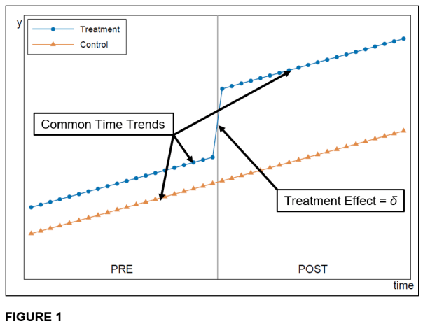
Let δ be the ATT (which is the same for everybody and constant over time). Note that ATT is given by the double difference DD, where,
The first difference sweeps out any unobserved fixed effects that characterize Treatment individuals. This leaves δ plus the time trend for the Treatment group.
The second difference (in parentheses) sweeps out unobserved effects associated with Control individuals. This leaves the time trend for the Control group.
The first difference minus the second difference then leaves δ, the ATT, assuming both groups have a common time trend. (Note how the “common trends” assumption is key to identifying δ.)
It is easily shown that, given the above assumptions, that OLS estimation of the regression specification below produces an unbiased estimate of δ.

A more realistic, three-period example
Now consider a more realistic example, close in spirit to what researchers actually encounter in practice. Let there be three groups, “Early Treatment”, “Late Treatment” and “Never Treated”; and three time periods, “Pre”, “Mid”, and “Post”.
FIGURE 2 motivates the following discussion.
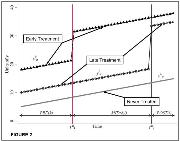
The Early Treatment group receives treatment at t*k (GB uses the k subscript to indicate early treatees).
The Late Treatment group receives treatment at t*l , t*l > t*k .
Suppose a researcher were to estimate the following 2WFE regression equation, where Dit is a dummy variable indicating whether individual i was treated at or before time t. For example, Dit = 0 and 1 for Late treatees at times “Mid” and “Post”, while Dit = 1 for Early treatees at times “Mid” and “Post”,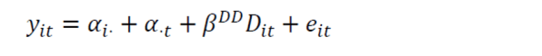 GB shows that the OLS estimate of βDD is a weighted average of all possible DD paired differences. One of those paired differences (cf. Equation 6 in GB) is
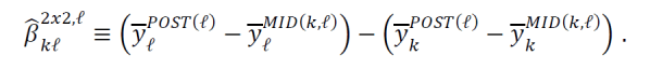 Note that in this case, the Early Treatment group (subscripted by k) can serve as a control group for the Late Treatment group because its treatment status does not change over the “Mid”/“Post” period. This particular paired difference ends up being important.
GB goes on to derive the following decomposition result: The probability limit of the OLS estimator of βDD consists of three components: VWATT is the Variance Weighted ATT, VWCT is the Variance Weighted Common Trends, and ΔATT is the change in individuals’ treatment effects that occurs over time, where the weights come from sample size and treatment variance.
When the common trends assumption is valid (VWCT=0), and the treatment effect is homogeneous both across individuals and within individuals over time, then the probability limit equals δ, the homogeneous treatment effect.
However, if treatment effects are heterogeneous, then even if the common trends assumption holds, estimation of the 2WFE specification will not equal the ATT. There are two sources of bias.
The first bias arise because OLS weights individual treatment effects differently depending on (i) the number of people who are treated and (ii) the timing of the treatment. This will introduce a bias if the size of the treatment effect is associated with either of these. However, this bias is not necessarily a bad thing. It is the byproduct of minimizing the variance of the estimator, so there are some efficiency gains that accompany this bias.
The second bias is associated with changes in the treatment effect over time, ΔATT. It’s entirely a bad thing.
Consider again the paired difference
The second term is the difference in outcomes for the Early treatees between the Post and Mid periods. Because Early treatees are treated for both of these periods, this difference should sweep away everything but the time trend if the treatment effect stays constant over time.
However, if treatment effects vary over time, say the benefits depreciate (or, alternatively, accumulate), the treatment effect will not be swept out. As a result, the change in the treatment effect will carry through to the respective DD estimate. As a result, the DD estimate will respectively over- or under-estimate the true treatment effect.
GB’s decomposition allows one to investigate this last type of bias. Towards that end, GB (along with Thomas Goldring and Austin Nichols) has written a Stata module called bacondecomp.
Application: Replication of Stevenson and Wolfers (2006)
To demonstate bacondecomp, GB replicates a result from the paper “Bargaining in the Shadow of the Law: Divorce Laws and Family Distress” by Betsey Stevenson and Justin Wolfers (S&W), published in The Quarterly Journal of Economics in 2006.
Among other things, S&W estimate the effect of state-level, no-fault divorce laws on female suicide. Over their sample period of 1964–1996, 37 US states gradually adopted no-fault divorce. 8 states had already done so, and 5 states never did.
[NOTE: The data and code to reproduce the results below are taken directly from the examples in the help file accompanying bacondecomp. They can be obtained by installing bacondecomp and then accessing the help documentation through Stata].
GB does not exactly reproduce S&W’s result, but uses a similar specification and obtains a similar result. In particular, he estimates the following regression
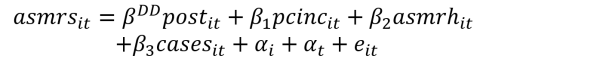 where asmrs is the suicide mortality rate per one million women; post is the treatment dummy variable (i.e., Dit); pcinc, asmrh, and cases are control variables for income, the homicide mortality rate, and the welfare case load; and αi and αt are individual and time fixed effects.
The 2WFE estimate of βDD is -2.52. In other words, this specification estimates that no-default divorce reform reduced female suicides by 2.52 fatalities per million women.
The bacondecomp command decomposes the 2WFE estimate of -2.52 into three separate components by treatment (T) and control (C) groups.
Timing_groups: Early treatees (T) versus Late treatees (C) & Late treatees (T) versus Early treatees (C).
Always_v_timing: Treatees (T) versus Always treated/Pre-reform states (C).
And Never_v_timing: Treatees (T) versus Never treated (C).
bacondecomp produces the following table, where “Beta” is the DD estimate for the respective group and “TotalWeight” represents its share in the overall estimated effect (-2.52). Notice that the sum of the products of “Beta” × “TotalWeight” ≈ the 2WFE estimate.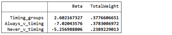
Conspiculously, the first group (Timing_groups) finds that no-fault divorce reform is associated with an increase in the female suicide rate (+2.60). In contrast, the latter two groups find a decrease (-7.02 and -5.26). This is indicative that there may be changes in treatment effects over time. If so, this would invalidate the difference-in-differences estimation framework.
Unfortunately, bacondecomp does not produce a corrected estimate of ATT. It is primarily useful for identifying a potential problem with time-varying treatment effects. As a result, it should be seen as complementing other approaches, such as the estimation procedures of de Chaisemartin and D’Haultfoeuille (see here), or an alternative approach such as an event study framework that includes dummies for each post-treatment period (see here).
Bob Reed is a professor of economics at the University of Canterbury in New Zealand. He is also co-organizer of the blogsite The Replication Network. He can be contacted at bob.reed@canterbury.ac.nz.
References
Goodman-Bacon, A., Goldring, T., & Nichols, A. (2019). bacondecomp: Stata module for decomposing difference-in-differences estimation with variation in treatment timing. https://ideas.repec.org/c/boc/bocode/s458676.html

Pingback: #StackBounty: #econometrics #difference-in-difference #control-group How to plot the graph for testing paralell trend for staggered DID? – TechUtils.in
Not sure what you are asking about “prioritizing for the treatment sample”. As I understand it, the treatment sample (and control sample) are changing over time which contributes to the time-varying nature of the treatment effect. PS Sorry for the slow response!
LikeLike