In Frequentist statistical inference, the p-value is used as a measure of how incompatible the data are with the null hypothesis.  When the null hypothesis is fixed at a point, the test statistic reports a distance from the sample statistic to this point. A low (high) p-value means that this distance is large (small), relative to the sampling variability. Hence, the p-value also reports this distance, but in a different scale, namely the scale of probability.

In a recent article published in Econometrics (“Interval-Based Hypothesis Testing and Its Applications to Economics and Finance”), we highlight the problems with the p-value criterion in concert with point null hypotheses.  We propose that researchers move to interval-based hypothesis testing instead.  While such a proposal is not new (Hodges and Lehmann, 1954) and such tests are being used in biostatistics and psychology (Welleck, 2010), it is virtually unknown to economics and business disciplines. In what follows, we highlight problems with the p-value criterion and show how they can be overcome by adopting interval-based hypothesis testing.

The first problem concerns economic significance; namely, whether the distance between the sample statistic and the point under the null has any economic importance. The p-value has nothing to say about this: it only reports whether the distance is large relative to the variability — not the relevance of the distance. It is certainly possible to have statistically significant results that are economically or operationally meaningless. 

The second problem is that the implied critical value of the test changes very little with sample size, while the test statistic generally increases with sample size. This is because the sampling distribution does not change, or does not change much. Stated differently, the distribution from which one obtains the critical value is (nearly) the same, regardless of how large or small sample size (or statistical power) is. 

And last but not least, since the population parameter can never be exactly equal to the null value under the point-null hypothesis, the sampling distribution under the null hypothesis is never realized or observed in reality. As a result, when a researcher calculates a t-statistic, it is almost certain that she obtains the value from a distribution under the alternative (a non-central t-distribution), and not from the distribution under the null (a central t-distribution). This can cause the critical value from the central distribution to be misleading, especially when the sample size is large.

Consider a simple t-test for H₀:θ=0, where θ represents the population mean. Assuming a random sample from a normal distribution with unknown standard deviation σ, the test statistic is t = n^0.5Xbar/σ where σ denotes the sample standard deviation. The test statistic follows a Student-t distribution with (n-1) degrees of freedom and non-centrality parameter λ=n^0.5θ/σ, denoted as t(n-1; λ). Under H₀, the t-statistic follows a central t-distribution with λ=0.

In reality, the value of θ cannot exactly and literally be 0. As Delong and Lang (1992) point out, “almost all tested null hypothesis in economics are false”. The consequence is that, with observational data, a t-statistic is (almost) always generated from a non-central t-distribution, not from a central one.

Suppose the value of θ was in fact 0.1 and that this value implies no economic or practical importance. That is, H₀ practically holds. Let us assume for simplicity that σ=1. When n = 10, the t-statistic is in fact generated from t(9; λ=0.316), not from t(9; λ=0). When the sample size is small — for example, 10 — the two distributions are very close, so the p-value can be a reasonable indicator for the evidence against H₀. When the sample size is larger, say 1000, the t-statistic is generated from t(999; λ=3.16). When it is 5000, it is generated from t(4999; λ=7.07). Under the point-null hypothesis, the distribution is fixed at t(n-1; λ=0). At this large sample size, every t-statistic is larger than the critical value at a conventional level; and every p-value is virtually equal to 0. Hence, although economically insignificant, a sample estimate of θ=0.1 will be statistically significant with a large t-statistic and a near-zero p-value.

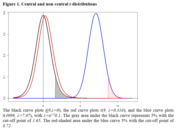
This situation is illustrated in Figure 1, where the black curve plots the central t-distribution; and red and blue curves show non-central distributions respectively for λ=0.316 and λ=7.07. The blue curve is an essentially a normal distribution, but for the purpose of illustration, we maintain it as a t-distribution with λ > 0. The point-null hypothesis fixes the sampling distribution at the black curve which is t(n-1; λ=0), so the 5% critical value does not change (no more than 1.645) regardless of sample size.

The consequence is that, when the value of  λ is as large as 7.07 with a large sample size, the null hypothesis is almost always rejected with the p-value virtually 0, even though θ=0.1 is economically negligible. The problem may not be serious when the sample size is small, but it is when the sample size is large. We now show how adopting an interval hypothesis allows one to overcome this problem.

Consider H₀: 0 < θ ≤ 0.5 against H₁: θ > 0.5. Let the value of θ = 0.5 be the minimum value of economic importance. Under the null hypothesis, the mean is economically negligible or practically no different from 0; while it makes a difference economically under H₁. This class of interval-based tests is called minimum-effect tests.

The decision rule is to reject H₀ at the 5% level if the t-statistic is greater than the critical value from t(n-1, λ=n^1/20.5) distribution. That is, the critical value increases with the sample size. If this distribution were the blue curve in Figure 1, the corresponding 5% critical value would be 8.72, indicated by the cut-off value corresponding to the red-shaded area.

In conducting an interval-based test, choosing the interval of economic significance is crucial for the credibility of the test. It should be set by the researcher, based on economic analysis or value judgment, desirably with a consensus from other researchers and ideally before she observes the data.

With such an interval hypothesis, a clear statement is made on the economic significance of the parameter and is taken into account for decision-making. In addition, the critical value and the sampling distribution of the test change with sample size; and the p-value is not necessarily a decreasing function of sample size.

As a practical illustration, we analyze the Halloween effect (Bouman and Jacobsen, 2002), where it is claimed that stock returns are consistently higher from the period of November to April. They fit a simple regression model of the form

            R_t = γ₀ + γ₁ D_t + u_t,

where R_t is stock return in percentage and D_t is a dummy variable which takes 1 from November to April; and 0 otherwise.

Using monthly data for a large number of stock markets around the world, Bouman and Jacobsen (2002; Table 1) report positive and statistically significant values of  γ₁. For the U.S. market using 344 monthly observations, they report that the estimated value of γ₁ is 0.96 with a t-statistic of 1.95.

Using daily data from 1950 to 2016 (16,819 observations), we replicate their results with an estimated value of γ₁=0.05 and a t-statistic of 3.44. For the point-null hypothesis H₀: γ₁ = 0; H₁: γ₁  > 0, we reject H₀ at the 5% level of significance for both monthly and daily data, with p-values of 0.026 and 0.0003 respectively. The Halloween effect is statistically clear and strong, especially when the sample size is larger.

Now we conduct minimum-effect tests. We assume that the stock return should be at least 1% higher per month during the period of November to April to be considered economically significance. This value is conservative considering trading costs and the volatility of the market.

The corresponding null and alternative hypotheses are H₀: 0 < γ₁ ≤ 1; H₁: γ₁ > 1. The 5% critical value of this test is 3.66 obtained from t(342, λ=2.06). On a daily basis, it is equivalent to H₀: 0 < γ₁ ≤ 0.05; H₁: γ₁ > 0.05, assuming 20 trading days per month. The 5% critical value of this test is 5.28 obtained from t(16,817, λ=3.60). For both cases, the null hypothesis of no economic significance cannot be rejected at the 5% level of significance. That is, the Halloween effect is found to be economically negligible with interval-based hypothesis testing.

In Figure 2, we present the Box-Whisker plot of the daily returns against D. It appears that there are a lot more outliers during the non-Halloween period, but the median and the quartile values are nearly identical for the two periods.

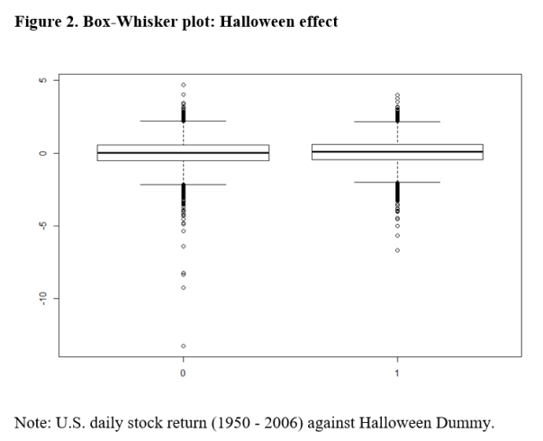
This plot provides further evidence that the Halloween effect is negligible, apart from these outliers. It is likely that the effect size estimates of the above Halloween regressions are over-stated by ignoring these outliers. This application highlights the problems of the point-null hypothesis and demonstrates how interval hypothesis testing can overcome them.

As Rao and Lovric (2016) argue, the paradigm of point-null hypothesis testing is no longer viable in the era of big data. Now is the time to adopt a new paradigm for statistical decision-making. In our article, we demonstrate that testing for an interval-null hypothesis can be a way forward.

Jae (Paul) Kim is a Professor of Finance in the Department of Finance at La Trobe University. Andrew Robinson is Director of the Centre of Excellence for Biosecurity Risk Analysis and Associate Professor in the School of Mathematics and Statistics, both at the University of Melbourne. Comments and/or questions about this blog can be directed to Professor Kim at J.Kim@latrobe.edu.au.

References

Bouman, S. Jacobsen, B. 2002. The Halloween Indicator, “Sell in May and Go Away”: Another Puzzle,  American Economic Review, 92(5), 1618-1635.

DeLong, J.B. and K. Lang, 1992, Are All Economic Hypotheses False? Journal of Political Economy, Vol. 100, No. 6, pp. 1257-72.

Hodges, J. L. Jr. and E.L. Lehmann 1954, Testing the Approximate Validity of Statistical Hypotheses, Journal of the Royal Statistical Society, Series B (Methodological), Vol. 16, No. 2, pp. 261–268.

Rao, C. R. and Lovric, M. M., 2016, Testing Point Null Hypothesis of a Normal Mean and the Truth: 21st Century Perspective, Journal of Modern Applied Statistical Methods, 15 (2), 2–21.

Wellek, S., 2010, Testing Statistical Hypotheses of Equivalence and Noninferiority, 2nd edition, CRC Press, New York.