NOTE: This blog is a repost of a blog that was previously published at the MAER-Net blogsite (see here)

Introduction

Random Effects (RE) versus Fixed Effects (FE) has a long and active debate history. More recently, a “Knapp–Hartung–like” version of FE—Unrestricted Weighted Least Squares (UWLS)—has entered the fray (Stanley & Doucouliagos, 2015, 2016). UWLS is simply conventional weighted least squares using inverse sampling variance weights. It produces identical coefficient estimates to FE, albeit with different standard errors.

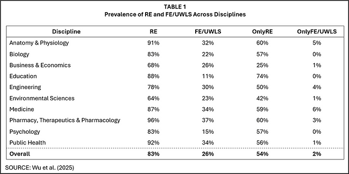
Among these approaches, RE is by far the most widely used. TABLE 1 is taken from a recently published study in Research Synthesis Methods that examined 1000 meta-analyses across 10 disciplines (Wu et al., 2025). In each and every discipline, RE was more widely employed than FE/UWLS. Moreover, when meta-analysts relied on only one estimator, that estimator was overwhelmingly RE.

Despite this widespread preference, the debate over RE versus FE/UWLS remains active, especially in contexts involving publication selection bias. In this blog, I highlight an additional reason to favor RE—one that has received little attention. The key idea is that a property of FE/UWLS that is often viewed as an advantage can, under realistic conditions, become a disadvantage.

The Context

There are multiple arguments that come into play in the RE versus FE/UWLS debate. Two are listed below.

RE is generally a more realistic framework. In economics and the social sciences, it is typically more plausible to assume that true effects vary across studies—as the RE model allows—than to assume a single common effect, as in FE. This likely explains why RE is the estimator of choice in most applied meta-analyses. However it needs to be noted that realism does not guarantee better performance. As Stanley and Doucouliagos (2023) illustrate, an empirically incorrect meta-analytic model can sometimes yield superior statistical results. Thus, even if the RE model more accurately reflects the data-generating process, that is not a decisive argument in its favor.

Recent evidence favors UWLS on goodness-of-fit grounds. Stanley et al. (2023) report that UWLS provides a better fit than RE for 67,308 meta-analyses from the Cochrane Database of Systematic Reviews (CDSR). However, in a separate paper, Sanghyun Hong and I challenge that conclusion.

These two points frame the broader discussion but are not my focus here. Instead, I examine a different issue—one that arises from the way FE/UWLS assigns weights.

Why FE/UWLS is thought to be better in the presence of publication selection bias

A frequently asserted argument in favor of FE/UWLS is that it performs better than RE when estimates are distorted by publication selection bias.

The logic is simple. Studies with large standard errors are most vulnerable to publication bias because they must report large, estimated effects to obtain statistical significance. More precise studies, with small standard errors, can be published even when their estimated effects are modest. As a result, small-SE studies are less distorted by selection and more representative of the underlying population of true effects. Because FE/UWLS assigns most of its weight to these highly precise—and thus less biased—studies, it is expected to produce pooled estimates that are both less biased and more efficient than RE.

Previous simulation work, including my own, supports this conclusion. In Hong & Reed, (2020) we found that WAAP—a method that, like FE/UWLS, prioritizes estimates with small standard errors—consistently outperformed RE on both bias and RMSE. Although that study did not directly compare FE/UWLS against RE, the underlying logic is the same: giving more weight to precise studies can mitigate the positive bias induced by publication selection.

Is it possible that previous simulations have it wrong?

Previous simulations may all be making a mistake. When generating primary study estimates, simulations typically assume that true effects are uncorrelated with the size of the standard errors. While that assumption may be valid for the population, it may not be warranted for a given sample.  

As simulations are typically constructed, heterogeneity is modeled by each replication drawing a new set of true effects from a population distribution. Every simulated meta-analysis therefore reflects a different random sample of true effects. Any chance correlation between true effects and standard errors in one replication will tend to get cancelled out when results are averaged over 1,000 or 10,000 simulations. In other words, the simulation design structurally forces the correlation between true effects and standard errors to be zero.

But in any given meta-analysis, we observe only a single realization of true effects—one draw, not thousands. In that realized sample, the correlation between true effects and standard errors need not be zero. When such correlations occur, estimators that place substantial weight on a small number of highly precise studies can yield realized estimates that differ markedly from what unconditional simulation averages would suggest.

The problem with giving large weights to a few studies

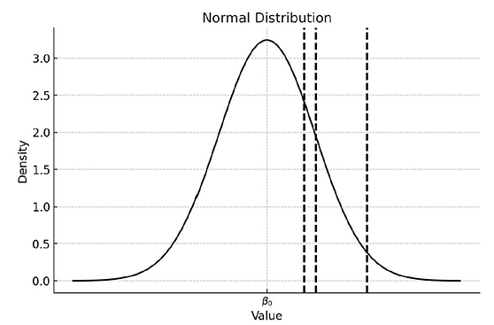
FIGURE 1 illustrates how estimators that place heavy weight on a small number of highly precise studies can yield misleading results.. The population of true effects is centered on β₀, but the studies with the smallest standard errors (indicated by the vertical lines) happen, in this particular sample, to lie well above β₀. If an estimator such as FE/UWLS heavily weights these three studies, they will exert disproportionate influence, pulling the pooled estimate upward.

FIGURE 1: Distribution of true effects

How often does a small number of studies dominate the overall estimate? In my experience of working with economics and social science data, quite often. TABLE 2 summarizes five recent meta-analyses in which I have been involved. Column 2 reports the number of studies; column 3 the percentage of total FE/UWLS weight assigned to the top three studies; and column 4 the corresponding I² values.

TABLE 2: Weights given to top 3 studies in selected meta-analyses

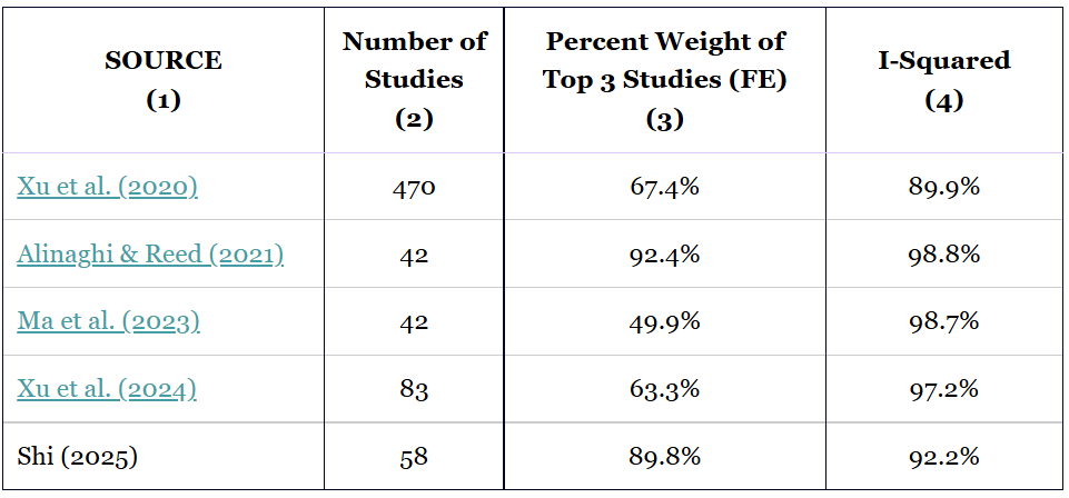
Across these meta-analyses, the top three studies receive anywhere from about 50% to over 90% of the total weight. Xu et al. (2020), for instance, contains 470 studies, yet just three of them account for more than two-thirds of the FE/UWLS weight. That concentration alone should raise concern: those few studies may not be representative of the broader distribution of true effects.

The problem becomes more serious when heterogeneity is high. The I² values for these studies range from 89.9% to 98.8%, which is typical in economics and the social sciences. Such values indicate that the true-effect distribution is extremely wide relative to sampling error. Under these conditions, it is entirely plausible that three randomly chosen studies (those with the smallest standard errors) could tilt the pooled estimate away from the population mean as in FIGURE 1. The concern with inverse sampling variance weighting in the presence of strong heterogeneity has long been noted (Hardy & Thompson, 1998; Song et al., 2001; Moreno et al., 2012).

Is this really a problem? Hard to say

The combination of (i) a small number of studies receiving a large share of the total weight and (ii) a highly dispersed distribution of true effects does not, by itself, guarantee a problem. These conditions only matter if the heavily weighted studies are unrepresentative of the underlying population of true effects.

The challenge is that this is extremely difficult to verify. We never observe the pre–publication-selection distribution of true effects. If we could, we could check directly whether the studies with the smallest standard errors differ meaningfully from the population. But in real meta-analysis, we only observe the post-selection distribution—the subset of results that survive publication filters. Consequently, we cannot distinguish whether unusual patterns arise because a few estimates are unrepresentatively drawn or because publication selection has distorted the observed distribution.

A simple example illustrates the problem. Suppose a researcher runs an Egger regression and obtains a positive coefficient on the standard error. Is this evidence of positive publication bias? Possibly. But it could equally reflect a situation where the most precise studies happen, by chance, to lie below the population mean, inducing a positive relationship between estimated effects and standard errors. The two explanations—publication bias versus sample unrepresentativeness—are observationally equivalent.

There is one case where the two explanations could be distinguished. If a researcher were confident of the sign of publication selection bias (positive/negative), then the coefficient on the standard error variable in an Egger regression should have the same sign. If the actual estimated coefficient has the opposite sign, this would be consistent with the “small standard error estimates are unrepresentative” hypothesis. Even then, such a finding could only establish existence of the problem, not extent. The problem could be lurking in many meta-analyses, but not identifiable either because the bias was in the same direction as publication selection, or because publication selection masked its existence.

How to show this in a simulation?

The challenge of illustrating this with a simulation is that this is a sample problem, arising from a one-off, random draw of observations taken from a distribution of true effects. A simulation of repeated, random draws would have the three most heavily weighted studies sometimes having true effects below the mean, and sometimes having true effects above the mean. Averaged over 1000 or more simulations, any sample correlations between standard errors and true effects would get washed out.

To address this problem, I impose a correlation between true effects and standard errors at the population level. This ensures that the simulated samples reflect the correlation between true effects and standard error that form the core of the argument above. The setup is therefore an imperfect but useful analogy for illustrating the dependency issue.

My simulation generates 100 meta-analyses, each containing 100 primary studies before any publication selection occurs. For every primary study, I draw a unique true effect from a normal distribution and assign a random error term with its own standard deviation. This ensures that some studies produce highly precise estimates, while others are much noisier.

I examine two versions of this setup.

1) Without publication selection bias: all study estimates enter the meta-analysis.

2) With publication selection bias: only statistically significant estimates are “published” and included.

This simple design captures the key features of applied meta-analysis—heterogeneity, varying precision, and selective reporting—and allows us to see clearly when inverse sampling variance weighting makes things better, and when it makes things worse.

Simulating correlation between effects and standard errors

The key line of code in my simulation program that generates correlation between effects and standard errors is given in the box below:

where

– “true_effect” is the true effect for a given primary study

– “mu” is the overall mean of the true-effect distribution

– “error_sd” is the standard deviation of errors in the DGP that produces individual observations in a given primary study. The larger the “error_sd”, the larger the standard error of the estimated effect for that primary study. The error SDs are assumed to be uniformly distributed.

– “tau” is the standard deviation of residual heterogeneity in true effects (after standardizing, it becomes the standard deviation of true effects)

– “corr” controls the extent to which true effects are related to the studies’ standard errors.

The idea is that true effects have a mean  and variance, but the true effects will be related to the standard errors of the estimated effects depending on the value of “corr”. (In the actual program, true_effect is transformed to keep its variance constant for different values of “corr”. )

When corr = 0, the simulation reflects the conventional assumption used in most published Monte Carlo studies: studies differ in their true effects, but those effects are unrelated to the studies’ precisions. This is the world where FE/UWLS typically performs well under publication bias.

 When corr ≠ 0, the story changes. Now the true effects and the standard errors move together, so the most precise studies may lie systematically above or below the population mean. In such samples, the estimates with the smallest standard errors are not representative of the full distribution of true effects. Yet FE/UWLS gives those same studies most of the weight—setting up exactly the situation in which inverse-variance weighting can produce biased results.

 This simple modification is designed to capture the real-world possibility that, in any single meta-analytic dataset, sampling variability and study design differences can jointly produce a correlation between effect sizes and their precisions.

 Example where FE/UWLS is better than RE

I begin by examining a baseline scenario: there is no publication selection bias and corr = 0, meaning true effects are unrelated to standard errors. This setup reflects the assumptions used in most existing Monte Carlo studies. As shown in the left panel of FIGURE 2, all three estimators—OLS, FE/UWLS, and RE—are unbiased. Their efficiencies, however, differ in the expected way: RE is most efficient, FE/UWLS somewhat less so, and OLS least precise.

 FIGURE 2: Distributions of Estimated Effects Without and With Publication Selection Bias (corr = 0)

The right panel of FIGURE 2 introduces publication selection bias while keeping corr = 0. Here, FE/UWLS performs best, exhibiting both lower bias and root mean square error than RE or OLS. This result reproduces the standard argument for preferring FE/UWLS under publication bias.

 Why does FE/UWLS perform best in this case? When publication selection is present, studies with large standard errors must have large, estimated effects to be statistically significant and thus included in the published literature. Consequently, these imprecise studies are systematically positively biased. More precise studies by contrast require only modest effects to reach significance, so their published results remain closer to the underlying true-effect distribution.

FE/UWLS succeeds in this setting precisely because it gives most of the weight to these highly precise, less biased studies. In a world where true effects and study precisions are uncorrelated, and where publication bias primarily distorts the noisy studies, inverse-sampling variance weighting helps correct that distortion.

Example where RE is better than FE/UWLS

However, the strength of FE/UWLS can also be its weakness. When only a few studies receive most of the weight—and when those studies are not representative—FE/UWLS’s main advantage becomes a liability.

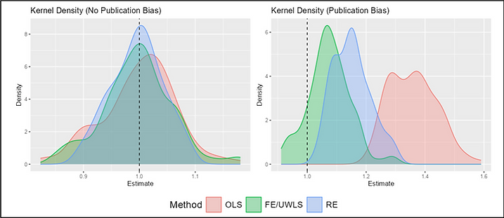
FIGURE 3 illustrates this situation. Here, estimated effects and standard errors are positively correlated in the pre-selection sample. As a result, the most precise studies tend to have smaller true effects, while the less precise studies tend to have larger ones. Under these conditions, weighting by inverse sampling variance pulls the pooled estimate downward, producing estimates that consistently lie below the population mean.

 FIGURE 3: Distributions of Estimated Effects Without and With Publication Selection Bias (corr > 0)

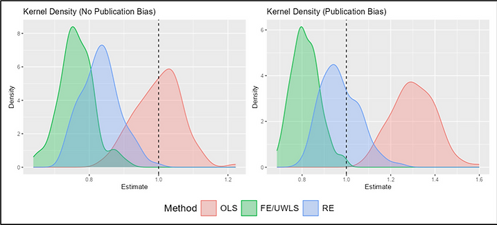
 As demonstrated in the left panel of FIGURE 3, without publication selection bias,

— OLS performs best, because it does not overweight the non-representative precise studies;

— RE performs reasonably well by partially shrinking the overly influential studies;

— FE/UWLS performs worst, because inverse-variance weighting amplifies the bias introduced by the correlation structure.

The right panel introduces publication selection bias, and the ranking shifts. Now two forces operate simultaneously:

1.     Publication bias, which pushes noisy estimates upward; and

2.    Correlation between effects and standard errors, which pushes inverse-variance weighted estimates downward.

In this tug-of-war, RE performs best because it partially adjusts for both influences. It moderates the publication-selection bias (which inflates the noisy studies) and avoids the extreme overweighting that would magnify the downward bias from the correlated true effects. FE/UWLS, by contrast, is pulled too far in one direction, and OLS too far in the other.

This example shows that once true effects and standard errors are correlated—a plausible situation in real meta-analytic datasets—the assumptions underpinning FE/UWLS’s superiority no longer hold. Under such conditions, RE can produce more reliable estimates.

A Shiny app to simulate more examples

Did I cherry pick this example? Absolutely! I chose parameter values that allowed me to illustrate a scenario where the correlation between true effects and standard errors clearly works against FE/UWLS. However, this outcome is confirmed using a wide range of plausible parameter settings.

Rather than taking my word for it, you can explore these patterns directly using the Shiny app developed for this blog (see here). The app allows you to vary key parameters—mu, tau, primary study sample sizes, and corr—by entering them in the simulation settings box (see below). You’ll find that RE is not universally better; in some settings FE/UWLS dominates. But once correlations between effects and standard errors are allowed, RE often provides the more reliable estimate.

Concluding thoughts

The following points summarize the main lessons of this blog.

The “few-studies problem” is fundamentally a sample-level problem. When a small number of highly precise studies dominate the weighting, FE/UWLS effectively becomes a “few-studies estimator.” If those few studies are not representative of the population distribution of true effects, the pooled estimate will be misleading. Standard simulation designs examine a data-generating process where there is no population correlation between true effects and standard errors (or sampling errors), which helps explain why earlier simulation studies often found FE/UWLS to outperform RE under publication selection bias.

Meta-analysts should routinely report weight concentration and heterogeneity. Simple diagnostics—such as the share of total weight carried by the top few studies and heterogeneity measures like I²—provide readers with a clearer sense of how vulnerable a meta-analysis is to the representativeness of a small subset of estimates. TABLE 2 illustrates the type of information that would be especially useful to include in applied work.

The same concerns raised here may may also apply to multi-level models. In a recent paper, Chen & Pustejovsky (2025) investigate methods to correct publication selection bias in the context of multi-level models. They conclude that a variant of the CHE estimator – something they call CHE-ISCW (Correlated and Hierarchical Effects model with Inverse Sampling Covariance Weights) — outperforms CHE. In a sense, CHE versus CHE-ISCW is a multi-level analog of the RE versus FE/UWLS comparison discussed here. As such, the “few studies” problem may apply to their comparison as well.

In conclusion, whether FE/UWLS or RE performs better depends critically on the representativeness of the small set of studies receiving most of the weight. The claim that FE/UWLS outperforms RE under publication selection bias implicitly assumes that, in the pre-publication-selection world, estimated effects are uncorrelated with their standard errors. This assumption may not hold in real samples. The presence of a few heavily weighted studies does not automatically mean RE is preferable—but it does support that possibility.

If nothing else, I hope this blog encourages greater attention to the risks that arise when a large amount of inferential weight is placed on a small number of studies.

NOTE: Bob Reed is Professor of Economics and the Director of UCMeta at the University of Canterbury. He can be reached at bob.reed@canterbury.ac.nz.

REFERENCES

Alinaghi, N., & Reed, W. R. (2020). Taxes and Economic Growth in OECD Countries: A Meta-analysis. Public Finance Review, 49(1), 3. https://doi.org/10.1177/1091142120961775

Chen, M., & Pustejovsky, J. E. (2025). Adapting methods for correcting selective reporting bias in meta-analysis of dependent effect sizes. Psychological Methods. https://doi.org/10.1037/met0000773

Hardy, R., & Thompson, S. G. (1998). Detecting and describing heterogeneity in meta-analysis. Statistics in Medicine, 17(8), 841. https://doi.org/10.1002/(sici)1097-0258(19980430)17:8<841::aid-sim781>3.0.co;2-d

Hong, S., & Reed, W. R. (2020). Using Monte Carlo experiments to select meta‐analytic estimators [Review of Using Monte Carlo experiments to select meta‐analytic estimators]. Research Synthesis Methods, 12(2), 192. Wiley. https://doi.org/10.1002/jrsm.1467

Ma, W., Hong, S., Reed, W. R., Duan, J., & Luu, P. Q. (2023). Yield effects of agricultural cooperative membership in developing countries: A meta‐analysis. Annals of Public and Cooperative Economics, 94(3), 761. https://doi.org/10.1111/apce.12411

Moreno, S. G., Sutton, A. J., Thompson, J. R., Ades, A. E., Abrams, K. R., & Cooper, N. J. (2012). A generalized weighting regression‐derived meta‐analysis estimator robust to small‐study effects and heterogeneity. Statistics in Medicine, 31(14), 1407. https://doi.org/10.1002/sim.4488

Shi, B. (2025). Unpublished research. University of Canterbury.

Song, F., Sheldon, T., Sutton, A. J., Abrams, K. R., & Jones, D. R. (2001). Methods for Exploring Heterogeneity in Meta-Analysis. Evaluation & the Health Professions, 24(2), 126. https://doi.org/10.1177/016327870102400203

Stanley, T. D., & Doucouliagos, H. (2015). Neither fixed nor random: weighted least squares meta‐analysis. Statistics in Medicine, 34(13), 2116. https://doi.org/10.1002/sim.6481

Stanley, T. D., & Doucouliagos, H. (2016). Neither fixed nor random: weighted least squares meta‐regression. Research Synthesis Methods, 8(1), 19. https://doi.org/10.1002/jrsm.1211

Stanley, T. D., & Doucouliagos, H. (2023). Correct standard errors can bias meta‐analysis. Research Synthesis Methods, 14(3), 515. https://doi.org/10.1002/jrsm.1631

Stanley, T. D., Ioannidis, J. P. A., Maier, M., Doucouliagos, H., Otte, W. M., & Bartoš, F. (2023). Unrestricted weighted least squares represent medical research better than random effects in 67,308 Cochrane meta-analyses. Journal of Clinical Epidemiology, 157, 53. Elsevier BV. https://doi.org/10.1016/j.jclinepi.2023.03.004

Wu, W., Duan, J., Reed, W. R., & Tipton, E. (2025). What can we learn from 1,000 meta-analyses across 10 different disciplines? Research Synthesis Methods, 1.

Xue, X., Reed, W. R., & Aert, R. C. M. van. (2024). Social capital and economic growth: A meta‐analysis. Journal of Economic Surveys, 39(4), 1395. https://doi.org/10.1111/joes.12660

Xue, X., Reed, W. R., & Menclova, A. (2020). Social capital and health: a meta-analysis [Review of Social capital and health: a meta-analysis]. Journal of Health Economics, 72, 102317. Elsevier BV. https://doi.org/10.1016/j.jhealeco.2020.102317