The Replication Network
Furthering the Practice of Replication in Economics
REED: Calculating Power After Estimation – Everybody Should Do This!
So your estimate is statistically insignificant and you’re wondering: Is it because the effect size is small, or does my study have too little power? In Tian et al. (2024), we propose a simple method for calculating statistical power after estimation (“post hoc power analysis”). While our application is targeted towards empirical studies in development economics, the method has many uses and is widely applicable across disciplines.
It is common to calculate statistical power before estimation (“a priori power analysis”). This allows researchers to determine the minimum sample size to achieve a given level of power for a given effect size. In contrast, post hoc power analysis is rarely done, and often discouraged (for example, see here).
There is a reason for this. The most common method for calculating post hoc power is flawed. In our paper, we explain the problem and demonstrate that our method successfully avoids this issue.
Before discussing our method, it is useful to review some of the reasons why one would want to calculate statistical power after estimation is completed.
When estimates are insignificant. All too commonly, statistical insignificance is taken as an indication that the true effect size is small, indistinguishable from zero. That may be the case. But it also may be the case that the statistical power of the study was insufficient to generate significance even if the true effect size were substantial. Knowing the statistical power of the regression equation that produced the estimated effect can help disentangle these two cases.
When estimates are significant. Post hoc power analysis can also be useful when estimates are statistically significant. In a recent paper, Ioannidis et al. (2017) analyzed “159 empirical economics literatures that draw upon 64,076 estimates of economic parameters reported in more than 6,700 empirical studies”. They calculated that the “median statistical power is 18%, or less.” Yet the great majority of these estimates were statistically significant. How can that be?
One explanation is Type M error. As elaborated in Gelman and Carlin (2014), Type M error is a phenomenon associated with random sampling . Estimated effects that are statistically significant will tend to be systematically larger than the population effect. If journals filter out insignificant estimates, then the estimates that get published are likely to overestimate the true effects.
Low statistical power is an indicator that Type M error may be present. Post hoc power analysis cannot definitively establish the presence of Type M error. The true effect may be substantially larger than the value assumed in the power analysis. But post hoc power analysis provides additional information that can help the researcher interpret the validity of estimates.
Our paper provide examples from actual randomized controlled trials that illustrate the cases above. We also demonstrate how post hoc power analysis can be useful to funding agencies to assess whether previously funded research met their stated power criteria.
Calculating statistical power. Mathematically, the calculation of statistical power (either a priori or post hoc) is straightforward. Let:
ES = an effect size
s.d.(ES_hat) = the standard deviation of estimated effects, ES_hat
τ = ES / s.d.(ES_hat)
tcritdf,1-α/2 = the critical t-value for a two-tailed t-test having df degrees of freedom and an associated significance level of α.
Given the above, one can use the equation below to calculate the power associated with any effect size ES:
(1) tvaluedf,1-Power = (tcritdf,1-α/2 – τ )
Equation (1) identifies the area of the t-distribution with df degrees of freedom that lies to the right of (tcritdf,1-α/2 – τ) (see FIGURE 1 in Tian et al., 2024). All that is required to calculate power is a given value for the effect size, ES; the standard deviation of estimated effect sizes, s.d.(ES_hat), which will depend on the estimator (e.g., OLS, OLS with clustered standard errors, etc.); the degrees of freedom df and the significance level α.
Most software packages that calculate statistical power essentially consist of estimating s.d.(ES_hat) based on inputs such as sample size, estimate of the standard deviation of the output variable, and other parameters of the estimation environment. This raises the question, why not directly estimate s.d.(ES_hat) with the standard error of the associated regression coefficient?
The SE-ES Method. We show that simply replacing s.d.(ES_hat) with the standard error of the estimated effect from the regression equation, s.e.(ES_hat), produces a useful, post hoc estimator of power. We call our method “SE-ES”, for Standard Error-Effect Size.
As long as s.e.(ES_hat) provides a reliable estimate of the variation in estimated effect sizes, SE-ES estimates of statistical power will perform well. As McKenzie and Ozier (2019) note, this condition generally appears to be the case.
Our paper provides a variety of Monte Carlo experiments to demonstrate the performance of the SE-ES method when (i) errors are independent and homoskedastic, and (ii) when they are clustered.
In the remainder of this blog, I present two simple R programs for calculating power after estimation. The first program produces a single-valued, post hoc estimate of statistical power. The user provides a given effect size, an alpha level, and the standard error of the estimated effect from the regression equation along with its degrees of freedom. This program is given below.
# Function to calculate power

power_function <- function(effect_size, standard_error, df, alpha) {

# This matches FIGURE 1 in Tian et al. (2024)
# "Power to the researchers: Calculating power after estimation"
#  Review of Development Economics
#  http://doi.org/10.1111/rode.13130

  t_crit <- qt(alpha / 2, df, lower.tail = FALSE)
  tau <- effect_size / standard_error
  t_value = t_crit - tau
  calculate_power <- pt(t_value, df, lower.tail = FALSE)

  return(calculate_power)
}
For example, if after running the power_function above, one wanted to calculate post hoc power for an effect size = 4, given a regression equation with 50 degrees of freedom where the associated coefficient had a standard error of 1.5, one would then run the chunk below.
# Example
alpha <- 0.05
df <- 50
effect_size <- 4
standard_error <- 1.5

power <- power_function(effect_size, standard_error, df, alpha)
print(power)
In this case, post hoc power is calculated to be 74.3% (see screen shot below).

Alternatively, rather than calculating a single power value, one might find it more useful to generate a power curve. To do that, you would first run the following program defining two functions: (i) the power_function (same as above), and (ii) the power_curve_function.
# Define the power function
power_function <- function(effect_size, standard_error, df, alpha) {
  # Calculate the critical t-value for the upper tail
  t_crit <- qt(alpha / 2, df, lower.tail = FALSE)
  qt(alpha / 2, df, lower.tail = FALSE)
  tau <- effect_size / standard_error
  t_value <- t_crit - tau
  calculate_power <- pt(t_value, df, lower.tail = FALSE)

  return(calculate_power)
}

# Define the power_curve_function
# Note that this uses the power_function above
power_curve_function <- function(max_effect_size, standard_error, df, alpha) {

  # Initialize vector to store results
  powers <- numeric(51)

  # Calculate step size for incrementing effect sizes
  d <- max_effect_size / 50

  # Create a sequence of 51 effect sizes
  # Each incremented by step size d
  effect_sizes <- seq(0, max_effect_size, by = d)

  # Loop through each effect size to calculate power
  for (i in 1:51) {
  effect_size <- effect_sizes[i]
  power_calculation <- power_function(effect_size, standard_error, df, alpha)
  powers[i] <- power_calculation
  }

  return(data.frame(EffectSize = effect_sizes, Power = powers))
}
Now suppose one wanted to create a power curve that corresponded to the previous example. You would still have to set alpha and provide values for df and the standard error from the estimated regression equation. But to generate a curve, you would also have to specify a maximum effect size.
The code below sets a maximum effect size of 10, and then creates a sequence of effect sizes from 0 to 10 in 50 equal steps.
# Define global parameters
alpha <- 0.05
df <- 50
standard_error <- 1.5
max_effect_size <- 10
d <- max_effect_size / 50
effect_sizes <- seq(0, max_effect_size, by = d)
Running the chunk below generates the power curve.
# Calculates vector to hold power values
powers <- numeric(51)

# Loop through each effect size to calculate power
for (i in 1:51) {
  effect_size <- effect_sizes[i]
  power_calculation <- power_function(effect_size, standard_error, df, alpha)
  powers[i] <- power_calculation
}

# Generate power curve data
power_data <- power_curve_function(max_effect_size, standard_error, df, alpha)

# Plot power curve
ggplot(power_data, aes(x = EffectSize, y = Power)) +
  geom_line() +
  labs(title = "Power Curve", x = "Effect Size", y = "Power") +
  theme_minimal()

# This shows the table of power values for each effect size
View(power_data)
The power curve is given below.
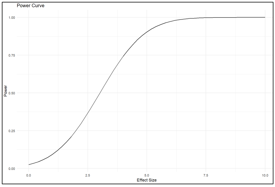
The last line of the chunk produces a dataframe that lists all the effect size-power value pairs. From there one can see that given a standard error of 1.5, the associated regression equation has an 80% probability of producing a statistically significant estimate when the effect size = 4.3.
The code above allows one to calculate power values and power curves for one’s own research. But perhaps its greatest value is that it allows one to conduct post hoc power analyses of estimated effects from other studies. All one needs to supply the programs is the standard error of the estimated effect and the associated degrees of freedom.
Limitation. The performance of the SE-ES method depends on the nature of the data and the type of estimator used for estimation. We found that it performed well when estimating linear models with clustered errors. However, one should be careful in applying the method to settings that are different from those investigated in our experiments. Accordingly, good practice would customize Tian et al.’s (2024) Monte Carlo simulations to see if the results carry over to data environments that represent the data at hand. To facilitate that, we have provided the respective codes and posted them at OSF here.
NOTE: Bob Reed is Professor of Economics and the Director of UCMeta at the University of Canterbury. He can be reached at bob.reed@canterbury.ac.nz.
REFERENCE
Tian, J., Coupé, T., Khatua, S., Reed, W. R., & Wood, B. D. K. (2024). Power to the researchers: Calculating power after estimation. Review of Development Economics, 1–35. https://doi.org/10.1111/rode.13130
COUPÉ: Why You Should Use Quarto to Make Your Papers More Replicable (and Your Life Easier!)
An important part of writing a paper is polishing the paper. You start with a first draft but then you find small mistakes, things to add or to remove. Which leads to redoing the analysis and a second, third and fourth draft of the paper. And then you get comments at seminars and from referees, further increasing the number of re-analyses and re-writes.
An annoying part of this process is that whenever you update your code and get new results, you also need to update the numbers and tables in your draft paper. Reformatting the same MS Word table for the 5th time is indeed frustrating. But it is also bad for the replicability of papers as it’s so easy to update the wrong column of a table or forget to update a number.
When writing my latest paper on the long term impact of war on life satisfaction, I discovered how Quarto allows one to solve these problems by enabling one to create code and paper from one document. It’s like writing your whole paper, text and code in Stata; or it’s like writing your whole paper, text and code in MS Word. True, R Markdown allows this too, but Quarto makes the process easier as it has MS Word-like drop down menus so you need to know less coding, making the learning curve substantially easier!
Whenever I now update the code for my latest paper, the text version gets updated automatically since every number and every table in the text is linked directly to the code! People who want to replicate the paper will also waste less time finding where in the code is the bit for table 5 from the paper, as the text is wrapped around the code so the code for table 5 is next to the text for table 5.
And there’s more! The R folder that has your code and datasets can easily be linked to Github so no more need to upload replication files to OSF or Harvard Dataverse!
And did I tell you documents in Quarto can be printed as pdf or word, and even html so you can publish your paper as a website: click here for an example.
How cool is that!
And did I tell you that you can use Quarto to create slides that are nicer than PPT and that can be linked directly to the code, so updating the code also means updating the numbers and tables in the slides?
Now I realize that, for the older reader, the cost of investing in R and Quarto might be prohibitive. But for the younger generation, there can only be one advice: drop Stata, drop Word, go for the free software that will make your life easier and science more replicable!
Tom Coupé is a Professor of Economics at the University of Canterbury, New Zealand. He can be contacted at tom.coupe@canterbury.ac.nz.
AoI*: “The Robustness Reproducibility of the American Economic Review” by Campbell et al. (2024)
[*AoI = “Articles of Interest” is a feature of TRN where we report abstracts of recent research related to replication and research integrity.]
ABSTRACT (taken from the article)
“We estimate the robustness reproducibility of key results from 17 non-experimental AER papers published in 2013 (8 papers) and 2022/23 (9 papers). We find that many of the results are not robust, with no improvement over time. The fraction of significant robustness tests (p<0.05) varies between 17% and 88% across the papers with a mean of 46%. The mean relative t/z-value of the robustness tests varies between 35% and 87% with a mean of 63%, suggesting selective reporting of analytical specifications that exaggerate statistical significance. A sample of economists (n=359) overestimates robustness reproducibility, but predictions are correlated with observed reproducibility.”
REFERENCE
COUPÉ: Why You Should Add a Specification Curve Analysis to Your Replications – and All Your Papers!
When making a conclusion based on a regression, we typically need to assume that the specification we use is the ‘correct’ specification. That is, we include the right control variables, use the right estimation technique, apply the right standard errors, etc. Unfortunately, most of the time theory doesn’t provide us with much guidance about what is the correct specification. To address such ‘model uncertainty’, many papers include robustness checks that show that conclusions remain the same whatever changes one makes to the main specification.
While when reading published papers, it’s rare to see specifications that do not support the main conclusions of a paper, many people who analyse data themselves quickly realize regression results often are much more fragile than what the published literature seems to suggest. For some, this even might lead to existential questions like “Why do I never get clean results, while everybody else does?”.
The recent literature based on ‘many-analyst’ projects confirms however that when different researchers are given the same research question and the same dataset, they often will come to different conclusions. Sometimes you can even observe such many-analyst project in real life: in a recent paper, my co-authors and I replicate several published papers that all use data from the same “Life in Transition Survey’ to estimate the long-term impact of war on life satisfaction. But while one paper concludes that there is a positive and significant effect, another concludes that there is a negative and significant effect, while a third one concludes there is no significant effect.
Interestingly, we can replicate the findings of these three papers so these differing findings cannot be explained by coding errors. Instead, it’s how these authors choose to specify their model that drove these differing results.
To illustrate the impact of specification choices on outcomes we use the specr R-package. To use specr, you indicate what are reasonable choices for your dependent variable, for your independent variable of interest, for your control variables, for your estimation model and for your sample restrictions. The general format is given below.
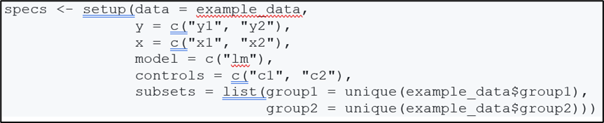
After specifying this snippet of code, specr will run all possible combinations and present them in two easy-to-understand graphs. For example, in our paper, we used 2 dependent variables (life satisfaction on a scale from 1-10 and life satisfaction on a scale from 1 to 5), one main variable of interest (injured or having relatives injured or killed during World War II), 5 models (based on how fixed effects and clusters were defined in 5 different published papers), 8 sets of controls (basic controls, additional war variables, income variables, other additional controls, etc.) and 4 datasets (the full dataset, respondents under 65 years old, those living in countries heavily affected by World War II, and under 65s living in heavily affected countries). This gave a total of 320 regression specifications.
The first graph produced by specr plots the specification curve, a curve showing all estimates of impact of the variable-of-interest on the outcome, and the standard errors, ordered from smallest to largest, giving an idea of the extent to which model uncertainty affects outcomes.

In the case of our paper, the specification curve showed a wide range of estimates of the impact of experiencing war on life satisfaction (from -0.5 to +0.25 on a scale of 1 to 5/10), with negative estimates often being significant (significant estimates are in red, grey is insignificant).
The second graph shows estimates by each specification-choice, illustrating what drives the heterogeneity in outcomes. In the case of our paper, we found that from the moment we controlled for a measure of income the estimate of war on life satisfaction became less negative and insignificant!

Given the potential importance of choices the researchers make on outcomes, it makes sense, when replicating a paper, to not just exactly replicating the authors specifications. Robustness checks in papers typically check how changing the specification in one dimension affects the outcome. A specification curve, however, allows to illustrate what happens if we look at all possible combinations of the robustness checks done in a paper. Moreover, programs like specr allow to easily check what happens if one adds other variables, include fixed effects or clusters at different level of aggregation, or restricts the sample in this or that way. In other words, you can illustrate the effects of model uncertainty in a much more comprehensive way than is typically done in a paper.
And why restrict this to replication papers only? Why not add a comprehensive specification curve to all your papers, showing the true extent of robustness in your own analysis too? In the process, you will perform a great service to many researchers, showing that they are not the only one getting estimates that are all over the place; and help science, by providing a more accurate picture of how sure we can be about what we know and what we do not know.
Tom Coupé is a Professor of Economics at the University of Canterbury, New Zealand. He can be contacted at tom.coupe@canterbury.ac.nz.
AoI*: “Mass Reproducibility and Replicability: A New Hope” by Brodeur et al. (2024)
[*AoI = “Articles of Interest” is a feature of TRN where we report abstracts of recent research related to replication and research integrity.]
ABSTRACT (taken from the article)
“This study pushes our understanding of research reliability by producing and replicating claims from 110 papers in leading economic and political science journals. The analysis involves com- putational reproducibility checks and robustness assessments. It reveals several patterns. First, we uncover a high rate of fully computationally reproducible results (over 85%). Second, excluding minor issues like missing packages or broken pathways, we uncover coding errors for about 25% of studies, with some studies containing multiple errors. Third, we test the robustness of the results to 5,511 re-analyses. We find a robustness reproducibility of about 70%. Robustness reproducibility rates are relatively higher for re-analyses that introduce new data and lower for re-analyses that change the sample or the definition of the dependent variable. Fourth, 52% of re-analysis effect size estimates are smaller than the original published estimates and the average statistical significance of a re-analysis is 77% of the original. Lastly, we rely on six teams of re- searchers working independently to answer eight additional research questions on the determinants of robustness reproducibility. Most teams find a negative relationship between replicators’ experience and reproducibility, while finding no relationship between reproducibility and the provision of intermediate or even raw data combined with the necessary cleaning codes.”
REFERENCE
COUPÉ: I Tried to Replicate a Paper with ChatGPT 4. Here is What I Learned.
Recent research suggests ChatGPT ‘aced the test of understanding in college economics’, ChatGPT ‘is effective in stock selection’ , that it “can predict future interest rate decisions” and that using ChatGPT “can yield more accurate predictions and enhance the performance of quantitative trading strategies’. ChatGPT 4 also does econometrics: when I submitted the dataset and description of one of my econometric case studies, ChatGPT was able to ‘read’ the document, run the regressions and correctly interpret the estimates.
But can it solve the replication crisis? That is, can you make ChatGPT 4 replicate a paper?
To find out the answer to this question, I selected a paper I recently tried to replicate without the help of ChatGPT, so I knew the data needed to replicate the paper were publicly available and the techniques used were common techniques that most graduate students would be able to do.[1]
I started by asking ChatGPT “can you replicate this paper : https://docs.iza.org/dp9017.pdf”.
ChatGPT answered : “I can’t directly access or replicate documents from external links.”
I got a similar answer when I asked it to download the dataset used in this paper – while it did find the dataset online, when asked to get the data, ChatGPT answered: ‘I can’t directly access or download files from the internet’.
LIMITATION 1: ChatGPT 4 cannot download papers or datasets from the internet.
So I decided to upload paper and the dataset myself – however ChatGPT informed me that ‘currently, the platform doesn’t support uploading files larger than 50 MB’. That can be problematic, the Life in Transition survey used for the paper, for example, is 200MB.
LIMITATION 2: ChatGPT 4 cannot handle big datasets (>50MB).
To help ChatGPT, I selected, from the survey, the data needed to construct the variables used in the paper and supplied ChatGPT with this much smaller dataset. I then asked ‘can you use this dataset to replicate the paper’. Rather than replicating the paper, ChatGPT reminded me of the general steps needed to analyse the data, that ‘we’re limited in executing complex statistical models directly here’, demonstrated how to do some analysis in Python and warned that ‘For an IV model, while I can provide guidance, you would need to implement it in a statistical software environment that supports IV estimations, such as R or Stata’.
While ChatGPT does provide R code when specifically asked for it, ChatGPT seems to prefer Python. Indeed, when I first tried to upload the dataset as an R dataset it answered [‘The current environment doesn’t support directly loading or manipulating R data files through Python libraries that aren’t available here, like rpy2’] So I then uploaded the data as a Stata dataset which it accepted. It’s also interesting ChatGPT recommends Stata and R for IV regressions even though IV regressions can be done in Python using the Statsmodels or linearmodels packages. What’s more, at a later stage ChatGPT did use Statsmodels to run the IV regression.
This focus on Python also limits the useability of ChatGPT to replicate papers for which the code is available – when I supplied the Stata code and paper for one of my own papers, it failed to translate and run the code into Python.
LIMITATION 3: ChatGPT 4 seems to prefer Python.
To make life easier for ChatGPT, I next shifted focus to one specific OLS regression: ‘can you try to replicate the first column of table 5 which is an OLS regression’.
ChatGPT again failed. Rather than focusing on column I which had the first stage of an IV regression, it took the second column with the IV results. And rather than running the regression, it provided some example code as it seemed unable to use the labels of the variables to construct the variables mentioned in the table and the paper. It is true that in the dataset the variable names were not informative (f.e. q721) but the labels attached to each question were informative so I made that explicit in the next step: ‘can you use the variable labels to find the variables corresponding to the ones uses in table 1’?
ChatGPT was still not able to create the variables and indicated that ‘Unfortunately, without direct access to the questionnaire or detailed variable labels and descriptions, I can provide only a general guide rather than specific variable names.’
I therefor upload the questionnaire itself. This helped ChatGPT a lot as it now discussed in more detail which variables were included. And while it still did not run the regression, it provided code in R rather than Python! Unfortunately, the code was still very far from what was needed: some needed variables were not included in the regression, some were included but not in the correct functional form, others that did not need to be included were included. ChatGPT clearly has difficulties to think about all the information mentioned in a paper when proposing a specification.
LIMITATION 4: ChatGPT 4 has trouble creating the relevant variables from variable names and labels.
Given its trouble with R, I asked ChatGPT to do the analysis Python. But that just lead to more trouble: ‘It looks like there was an issue converting the q722 variable, which represents life satisfaction, directly to a float. This issue can occur if the variable includes non-numeric values or categories that cannot be easily converted to numbers (e.g., “Not stated” or other text responses).’ Papers often do not explicitly state how they handle missing values and ChatGPT did not suggest focusing on ‘meaningful’ observations only. Once I indicated only values between 0 and 10 should be used, ChatGPT was able to use the life satisfaction variable but ran into trouble again when it checked other categorical variables.
LIMITATION 5: ChatGPT 4 gets into trouble when some part of the data processing is not fully described.
I next checked some other explanatory variables. The ‘network’ variable was based on a combination of two variables. ChatGPT, rather than using the paper to find how to construct the variable, described how such variable can be generated in general. Only after I reminded ChatGPT that ‘the paper clearly describes how the network variable was created’, ChatGPT created the variable correctly.
LIMITATION 6: ChatGPT 4 needs to be reminded to see the ‘big picture’ and consider all the information provided in the paper.
Finally, for the ‘minority’ variable one needed to check whether the language spoken by the mother of the respondent was an official language of the country where the respondent lives. ChatGPT used its knowledge of official languages to create a variable that suggested 97% of the sample belonged to a minority (against about 14% according to the paper’s summary statistics) but realized this was probably a mistake – it noted ‘this high percentage of respondents classified as linguistic minorities might suggest a need to review the mapping of countries to their official languages or the accuracy and representation of mother’s language data ‘
After this I gave up and concluded that while ChatGPT 4 can read files, analyse datasets and even run and interpret regressions, it is still very far from being able to be of much help while replicating a paper. That’s bad news for the replication crisis, but good news for those doing replications: there is still some time before those doing replications will be out of jobs!
CONCLUSION: ChatGPT 4 does not destroy replicators’ jobs (yet)
Full transcripts of my conversation with ChatGPT can be found here.
Tom Coupé is a Professor of Economics at the University of Canterbury, New Zealand. He can be contacted at tom.coupe@canterbury.ac.nz.
[1] For a paper analysing how wars affect happiness, my co-authors and I tried to replicate 5 papers, the results can be found here,
AoI*: “What Is the False Discovery Rate in Empirical Research?” by Engsted (2024)
[*AoI = “Articles of Interest” is a feature of TRN where we report abstracts of recent research related to replication and research integrity.]
ABSTRACT (taken from the article)
“A scientific discovery in empirical research, e.g., establishing a causal relationship between two variables, is typically based on rejecting a statistical null hypothesis of no relationship. What is the probability that such a rejection is a mistake? This probability is not controlled by the significance level of the test which is typically set at 5 percent. Statistically, the ‘False Discovery Rate’ (FDR) is the fraction of null rejections that are false. FDR depends on the significance level, the power of the test, and the prior probability that the null is true. All else equal, the higher the prior probability, the higher is the FDR. Economists have different views on how to assess this prior probability. I argue that for both statistical and economic reasons, the prior probability of the null should in general be quite high and, thus, the FDR in empirical economics is high, i.e., substantially higher than 5 percent. This may be a contributing factor behind the replication crisis that also haunts economics. Finally, I discuss conventional and newly proposed stricter significance thresholds and, more generally, the problems that passively observed economic and social science data pose for the traditional statistical testing paradigm.”
REFERENCE

WESSELBAUM: JCRE – An Outlet for Your Replications
Posted on by replicationnetwork
Leave a Comment
Replication studies play a crucial role in economics by ensuring the reliability, validity, and robustness of research findings. In an era where policy decisions and societal interventions heavily rely on economic research, the ability to replicate and validate research findings is important for making informed decisions and advancing knowledge. Replications in economics became more mainstream after the 2016 influential paper by Colin Camerer, Anna Dreber, and others published in Science. This paper replicated 18 studies from the AER and QJE published between 2011 and 2014. In only 61% (11 out of 18) of these, the replication found a significant effect in the same direction as in the original study.
Replication studies serve as a cornerstone of scientific integrity and transparency. Economics, like other empirical sciences, relies on data-driven analysis to draw conclusions about complex economic phenomena. However, the validity of these conclusions can often be challenged due to various factors such as data limitations, methodological choices, or even unintentional errors. By replicating papers, researchers can verify whether the original findings hold under different conditions, datasets, or methodologies. This process not only enhances the credibility of the research but also fosters trust.
Replications contribute to the cumulative nature of knowledge. Many economic theories and empirical results build upon earlier findings. However, the reliability of these findings can sometimes be uncertain, especially when they are based on limited samples or specific contexts. Replication studies allow researchers to confirm whether the findings are generalizable across different populations, time periods, or geographical regions. This cumulative process helps in refining theories, identifying boundaries, and uncovering inconsistencies that may require further investigation.
Additionally, replication studies encourage openness and collaboration within the economics community. They promote constructive dialogue among researchers about the strengths and limitations of different approaches and methodologies. By openly discussing replication efforts and their outcomes, we can collectively enhance research practices, improve data transparency, and foster a culture of quality assurance in economic research.
While some Journals (for example the Journal of Applied Econometrics, JPE: Micro, JESA, or Empirical Economics) publish replication studies, the new journal “Journal of Comments and Replications in Economics” (JCRE) aims to be the premier outlet for articles that comment on or replicate previously published articles.
Because many journals are reluctant to publish comments and replications, JCRE was founded to provide an outlet for research that explores whether published results are correct, robust, and/or generalizable and to publish replications defined as any study that directly addresses the reliability of a specific claim from a previously published study.
The editorial board of JCRE consists of W. Robert Reed (University of Canterbury), Marianne Saam (University of Hamburg), and myself (University of Otago). As editors, we are supported by the Leibniz Information Centre for Economics (ZBW) and the German Research Foundation (DFG).
Our advisory board consists of the following outstanding scholars: David Autor (MIT), Anna Dreber Almenberg (Stockholm School of Economics), Richard Easterlin (USC), Edward Leamer (UCLA), David Roodman (Open Philanthropy), and Jeffrey Wooldridge (MSU).
In conclusion, replication studies are indispensable in economics for several compelling reasons: they uphold scientific rigor and transparency, contribute to the cumulative advancement of knowledge, help identify biases and flaws in research, and promote openness and collaboration among researchers. We believe that with the increase in the availability of large data sets, the advancements in computer power, and the development of new econometric tools, the importance of replicating and validating research findings will only grow. To this end, we invite you to submit your replication studies to the JCRE and promote the Journal in your networks and among your students.
For more information about JCRE, click here.
Dennis Wesselbaum is Associate Professor of Economics at the University of Otago in New Zealand, and Co-Editor of the Journal of Comments and Replications in Economics (JCRE). He can be contacted at dennis.wesselbaum@otago.ac.nz.
Category: GUEST BLOGS Tags: Comments, economics, Journal, Journal policies, Publication, replications