The Replication Network
Furthering the Practice of Replication in Economics
AoI*: “Computational Reproducibility and Robustness of Empirical Economics and Political Science Research”
[*AoI = “Articles of Interest” is a feature of TRN where we report abstracts of recent research related to replication and research integrity.]
ABSTRACT (taken from the article)
“This systematic and large-scale reproduction effort tests the reproducibility and robustness of economics and political science. We reproduced original analyses and conducted robustness checks of 110 articles recently published in leading economics and political science journals (all of which have mandatory data and code sharing policies). We found that over 85% of published claims were computationally reproducible. In robustness checks, our re-analyses lead to 72% of statistically significant estimates to remain significant and in the same direction, and the median reproduced effect size is (nearly) the same as the originally published effect size (that is, 99% of the published effect size). Additionally, six independent research teams examined 12 prespecified hypotheses about determinants of robustness. Research teams with more experience found lower levels of robustness, but robustness correlated with neither author characteristics nor data availability.”
REFERENCE
Brodeur, A., Cook, N., Mikola, D., Fiala, L., & Heyes, A. (2026). Computational Reproducibility and Robustness of Empirical Economics and Political Science Research. Nature.
REED: Another Reason to Prefer Random Effects Over Fixed Effects/UWLS Meta-Analysis
NOTE: This blog is a repost of a blog that was previously published at the MAER-Net blogsite (see here)
Introduction
Random Effects (RE) versus Fixed Effects (FE) has a long and active debate history. More recently, a “Knapp–Hartung–like” version of FE—Unrestricted Weighted Least Squares (UWLS)—has entered the fray (Stanley & Doucouliagos, 2015, 2016). UWLS is simply conventional weighted least squares using inverse sampling variance weights. It produces identical coefficient estimates to FE, albeit with different standard errors.
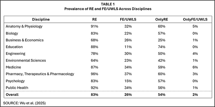
Among these approaches, RE is by far the most widely used. TABLE 1 is taken from a recently published study in Research Synthesis Methods that examined 1000 meta-analyses across 10 disciplines (Wu et al., 2025). In each and every discipline, RE was more widely employed than FE/UWLS. Moreover, when meta-analysts relied on only one estimator, that estimator was overwhelmingly RE.
Despite this widespread preference, the debate over RE versus FE/UWLS remains active, especially in contexts involving publication selection bias. In this blog, I highlight an additional reason to favor RE—one that has received little attention. The key idea is that a property of FE/UWLS that is often viewed as an advantage can, under realistic conditions, become a disadvantage.
The Context
There are multiple arguments that come into play in the RE versus FE/UWLS debate. Two are listed below.
RE is generally a more realistic framework. In economics and the social sciences, it is typically more plausible to assume that true effects vary across studies—as the RE model allows—than to assume a single common effect, as in FE. This likely explains why RE is the estimator of choice in most applied meta-analyses. However it needs to be noted that realism does not guarantee better performance. As Stanley and Doucouliagos (2023) illustrate, an empirically incorrect meta-analytic model can sometimes yield superior statistical results. Thus, even if the RE model more accurately reflects the data-generating process, that is not a decisive argument in its favor.
Recent evidence favors UWLS on goodness-of-fit grounds. Stanley et al. (2023) report that UWLS provides a better fit than RE for 67,308 meta-analyses from the Cochrane Database of Systematic Reviews (CDSR). However, in a separate paper, Sanghyun Hong and I challenge that conclusion.
These two points frame the broader discussion but are not my focus here. Instead, I examine a different issue—one that arises from the way FE/UWLS assigns weights.
Why FE/UWLS is thought to be better in the presence of publication selection bias
A frequently asserted argument in favor of FE/UWLS is that it performs better than RE when estimates are distorted by publication selection bias.
The logic is simple. Studies with large standard errors are most vulnerable to publication bias because they must report large, estimated effects to obtain statistical significance. More precise studies, with small standard errors, can be published even when their estimated effects are modest. As a result, small-SE studies are less distorted by selection and more representative of the underlying population of true effects. Because FE/UWLS assigns most of its weight to these highly precise—and thus less biased—studies, it is expected to produce pooled estimates that are both less biased and more efficient than RE.
Previous simulation work, including my own, supports this conclusion. In Hong & Reed, (2020) we found that WAAP—a method that, like FE/UWLS, prioritizes estimates with small standard errors—consistently outperformed RE on both bias and RMSE. Although that study did not directly compare FE/UWLS against RE, the underlying logic is the same: giving more weight to precise studies can mitigate the positive bias induced by publication selection.
Is it possible that previous simulations have it wrong?
Previous simulations may all be making a mistake. When generating primary study estimates, simulations typically assume that true effects are uncorrelated with the size of the standard errors. While that assumption may be valid for the population, it may not be warranted for a given sample.
As simulations are typically constructed, heterogeneity is modeled by each replication drawing a new set of true effects from a population distribution. Every simulated meta-analysis therefore reflects a different random sample of true effects. Any chance correlation between true effects and standard errors in one replication will tend to get cancelled out when results are averaged over 1,000 or 10,000 simulations. In other words, the simulation design structurally forces the correlation between true effects and standard errors to be zero.
But in any given meta-analysis, we observe only a single realization of true effects—one draw, not thousands. In that realized sample, the correlation between true effects and standard errors need not be zero. When such correlations occur, estimators that place substantial weight on a small number of highly precise studies can yield realized estimates that differ markedly from what unconditional simulation averages would suggest.
The problem with giving large weights to a few studies
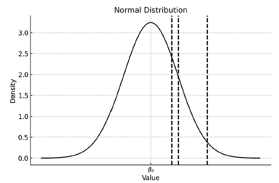
FIGURE 1 illustrates how estimators that place heavy weight on a small number of highly precise studies can yield misleading results.. The population of true effects is centered on β₀, but the studies with the smallest standard errors (indicated by the vertical lines) happen, in this particular sample, to lie well above β₀. If an estimator such as FE/UWLS heavily weights these three studies, they will exert disproportionate influence, pulling the pooled estimate upward.
FIGURE 1: Distribution of true effects
How often does a small number of studies dominate the overall estimate? In my experience of working with economics and social science data, quite often. TABLE 2 summarizes five recent meta-analyses in which I have been involved. Column 2 reports the number of studies; column 3 the percentage of total FE/UWLS weight assigned to the top three studies; and column 4 the corresponding I² values.
TABLE 2: Weights given to top 3 studies in selected meta-analyses
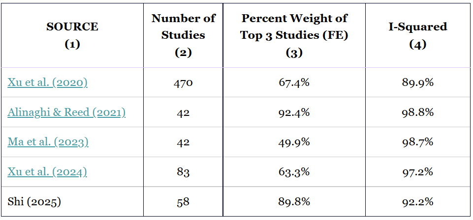
Across these meta-analyses, the top three studies receive anywhere from about 50% to over 90% of the total weight. Xu et al. (2020), for instance, contains 470 studies, yet just three of them account for more than two-thirds of the FE/UWLS weight. That concentration alone should raise concern: those few studies may not be representative of the broader distribution of true effects.
The problem becomes more serious when heterogeneity is high. The I² values for these studies range from 89.9% to 98.8%, which is typical in economics and the social sciences. Such values indicate that the true-effect distribution is extremely wide relative to sampling error. Under these conditions, it is entirely plausible that three randomly chosen studies (those with the smallest standard errors) could tilt the pooled estimate away from the population mean as in FIGURE 1. The concern with inverse sampling variance weighting in the presence of strong heterogeneity has long been noted (Hardy & Thompson, 1998; Song et al., 2001; Moreno et al., 2012).
Is this really a problem? Hard to say
The combination of (i) a small number of studies receiving a large share of the total weight and (ii) a highly dispersed distribution of true effects does not, by itself, guarantee a problem. These conditions only matter if the heavily weighted studies are unrepresentative of the underlying population of true effects.
The challenge is that this is extremely difficult to verify. We never observe the pre–publication-selection distribution of true effects. If we could, we could check directly whether the studies with the smallest standard errors differ meaningfully from the population. But in real meta-analysis, we only observe the post-selection distribution—the subset of results that survive publication filters. Consequently, we cannot distinguish whether unusual patterns arise because a few estimates are unrepresentatively drawn or because publication selection has distorted the observed distribution.
A simple example illustrates the problem. Suppose a researcher runs an Egger regression and obtains a positive coefficient on the standard error. Is this evidence of positive publication bias? Possibly. But it could equally reflect a situation where the most precise studies happen, by chance, to lie below the population mean, inducing a positive relationship between estimated effects and standard errors. The two explanations—publication bias versus sample unrepresentativeness—are observationally equivalent.
There is one case where the two explanations could be distinguished. If a researcher were confident of the sign of publication selection bias (positive/negative), then the coefficient on the standard error variable in an Egger regression should have the same sign. If the actual estimated coefficient has the opposite sign, this would be consistent with the “small standard error estimates are unrepresentative” hypothesis. Even then, such a finding could only establish existence of the problem, not extent. The problem could be lurking in many meta-analyses, but not identifiable either because the bias was in the same direction as publication selection, or because publication selection masked its existence.
How to show this in a simulation?
The challenge of illustrating this with a simulation is that this is a sample problem, arising from a one-off, random draw of observations taken from a distribution of true effects. A simulation of repeated, random draws would have the three most heavily weighted studies sometimes having true effects below the mean, and sometimes having true effects above the mean. Averaged over 1000 or more simulations, any sample correlations between standard errors and true effects would get washed out.
To address this problem, I impose a correlation between true effects and standard errors at the population level. This ensures that the simulated samples reflect the correlation between true effects and standard error that form the core of the argument above. The setup is therefore an imperfect but useful analogy for illustrating the dependency issue.
My simulation generates 100 meta-analyses, each containing 100 primary studies before any publication selection occurs. For every primary study, I draw a unique true effect from a normal distribution and assign a random error term with its own standard deviation. This ensures that some studies produce highly precise estimates, while others are much noisier.
I examine two versions of this setup.
1) Without publication selection bias: all study estimates enter the meta-analysis.
2) With publication selection bias: only statistically significant estimates are “published” and included.
This simple design captures the key features of applied meta-analysis—heterogeneity, varying precision, and selective reporting—and allows us to see clearly when inverse sampling variance weighting makes things better, and when it makes things worse.
Simulating correlation between effects and standard errors
The key line of code in my simulation program that generates correlation between effects and standard errors is given in the box below:

where
– “true_effect” is the true effect for a given primary study
– “mu” is the overall mean of the true-effect distribution
– “error_sd” is the standard deviation of errors in the DGP that produces individual observations in a given primary study. The larger the “error_sd”, the larger the standard error of the estimated effect for that primary study. The error SDs are assumed to be uniformly distributed.
– “tau” is the standard deviation of residual heterogeneity in true effects (after standardizing, it becomes the standard deviation of true effects)
– “corr” controls the extent to which true effects are related to the studies’ standard errors.
The idea is that true effects have a mean and variance, but the true effects will be related to the standard errors of the estimated effects depending on the value of “corr”. (In the actual program, true_effect is transformed to keep its variance constant for different values of “corr”. )
When corr = 0, the simulation reflects the conventional assumption used in most published Monte Carlo studies: studies differ in their true effects, but those effects are unrelated to the studies’ precisions. This is the world where FE/UWLS typically performs well under publication bias.
When corr ≠ 0, the story changes. Now the true effects and the standard errors move together, so the most precise studies may lie systematically above or below the population mean. In such samples, the estimates with the smallest standard errors are not representative of the full distribution of true effects. Yet FE/UWLS gives those same studies most of the weight—setting up exactly the situation in which inverse-variance weighting can produce biased results.
This simple modification is designed to capture the real-world possibility that, in any single meta-analytic dataset, sampling variability and study design differences can jointly produce a correlation between effect sizes and their precisions.
Example where FE/UWLS is better than RE
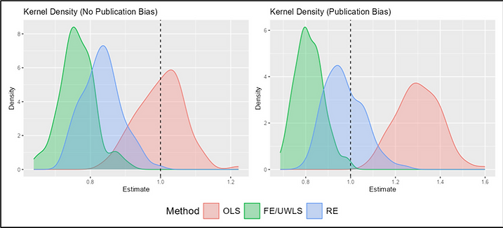
I begin by examining a baseline scenario: there is no publication selection bias and corr = 0, meaning true effects are unrelated to standard errors. This setup reflects the assumptions used in most existing Monte Carlo studies. As shown in the left panel of FIGURE 2, all three estimators—OLS, FE/UWLS, and RE—are unbiased. Their efficiencies, however, differ in the expected way: RE is most efficient, FE/UWLS somewhat less so, and OLS least precise.
FIGURE 2: Distributions of Estimated Effects Without and With Publication Selection Bias (corr = 0)
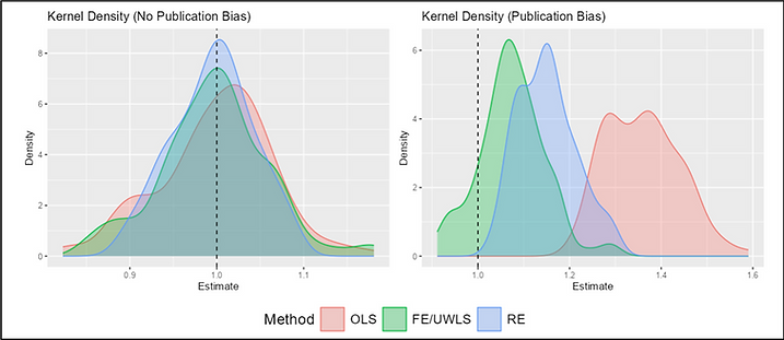
The right panel of FIGURE 2 introduces publication selection bias while keeping corr = 0. Here, FE/UWLS performs best, exhibiting both lower bias and root mean square error than RE or OLS. This result reproduces the standard argument for preferring FE/UWLS under publication bias.
Why does FE/UWLS perform best in this case? When publication selection is present, studies with large standard errors must have large, estimated effects to be statistically significant and thus included in the published literature. Consequently, these imprecise studies are systematically positively biased. More precise studies by contrast require only modest effects to reach significance, so their published results remain closer to the underlying true-effect distribution.
FE/UWLS succeeds in this setting precisely because it gives most of the weight to these highly precise, less biased studies. In a world where true effects and study precisions are uncorrelated, and where publication bias primarily distorts the noisy studies, inverse-sampling variance weighting helps correct that distortion.
Example where RE is better than FE/UWLS
However, the strength of FE/UWLS can also be its weakness. When only a few studies receive most of the weight—and when those studies are not representative—FE/UWLS’s main advantage becomes a liability.
FIGURE 3 illustrates this situation. Here, estimated effects and standard errors are positively correlated in the pre-selection sample. As a result, the most precise studies tend to have smaller true effects, while the less precise studies tend to have larger ones. Under these conditions, weighting by inverse sampling variance pulls the pooled estimate downward, producing estimates that consistently lie below the population mean.
FIGURE 3: Distributions of Estimated Effects Without and With Publication Selection Bias (corr > 0)
As demonstrated in the left panel of FIGURE 3, without publication selection bias,
— OLS performs best, because it does not overweight the non-representative precise studies;
— RE performs reasonably well by partially shrinking the overly influential studies;
— FE/UWLS performs worst, because inverse-variance weighting amplifies the bias introduced by the correlation structure.
The right panel introduces publication selection bias, and the ranking shifts. Now two forces operate simultaneously:
1. Publication bias, which pushes noisy estimates upward; and
2. Correlation between effects and standard errors, which pushes inverse-variance weighted estimates downward.
In this tug-of-war, RE performs best because it partially adjusts for both influences. It moderates the publication-selection bias (which inflates the noisy studies) and avoids the extreme overweighting that would magnify the downward bias from the correlated true effects. FE/UWLS, by contrast, is pulled too far in one direction, and OLS too far in the other.
This example shows that once true effects and standard errors are correlated—a plausible situation in real meta-analytic datasets—the assumptions underpinning FE/UWLS’s superiority no longer hold. Under such conditions, RE can produce more reliable estimates.
A Shiny app to simulate more examples
Did I cherry pick this example? Absolutely! I chose parameter values that allowed me to illustrate a scenario where the correlation between true effects and standard errors clearly works against FE/UWLS. However, this outcome is confirmed using a wide range of plausible parameter settings.
Rather than taking my word for it, you can explore these patterns directly using the Shiny app developed for this blog (see here). The app allows you to vary key parameters—mu, tau, primary study sample sizes, and corr—by entering them in the simulation settings box (see below). You’ll find that RE is not universally better; in some settings FE/UWLS dominates. But once correlations between effects and standard errors are allowed, RE often provides the more reliable estimate.
Concluding thoughts
The following points summarize the main lessons of this blog.
The “few-studies problem” is fundamentally a sample-level problem. When a small number of highly precise studies dominate the weighting, FE/UWLS effectively becomes a “few-studies estimator.” If those few studies are not representative of the population distribution of true effects, the pooled estimate will be misleading. Standard simulation designs examine a data-generating process where there is no population correlation between true effects and standard errors (or sampling errors), which helps explain why earlier simulation studies often found FE/UWLS to outperform RE under publication selection bias.
Meta-analysts should routinely report weight concentration and heterogeneity. Simple diagnostics—such as the share of total weight carried by the top few studies and heterogeneity measures like I²—provide readers with a clearer sense of how vulnerable a meta-analysis is to the representativeness of a small subset of estimates. TABLE 2 illustrates the type of information that would be especially useful to include in applied work.
The same concerns raised here may may also apply to multi-level models. In a recent paper, Chen & Pustejovsky (2025) investigate methods to correct publication selection bias in the context of multi-level models. They conclude that a variant of the CHE estimator – something they call CHE-ISCW (Correlated and Hierarchical Effects model with Inverse Sampling Covariance Weights) — outperforms CHE. In a sense, CHE versus CHE-ISCW is a multi-level analog of the RE versus FE/UWLS comparison discussed here. As such, the “few studies” problem may apply to their comparison as well.
In conclusion, whether FE/UWLS or RE performs better depends critically on the representativeness of the small set of studies receiving most of the weight. The claim that FE/UWLS outperforms RE under publication selection bias implicitly assumes that, in the pre-publication-selection world, estimated effects are uncorrelated with their standard errors. This assumption may not hold in real samples. The presence of a few heavily weighted studies does not automatically mean RE is preferable—but it does support that possibility.
If nothing else, I hope this blog encourages greater attention to the risks that arise when a large amount of inferential weight is placed on a small number of studies.
NOTE: Bob Reed is Professor of Economics and the Director of UCMeta at the University of Canterbury. He can be reached at bob.reed@canterbury.ac.nz.
REFERENCES
Alinaghi, N., & Reed, W. R. (2020). Taxes and Economic Growth in OECD Countries: A Meta-analysis. Public Finance Review, 49(1), 3. https://doi.org/10.1177/1091142120961775
Chen, M., & Pustejovsky, J. E. (2025). Adapting methods for correcting selective reporting bias in meta-analysis of dependent effect sizes. Psychological Methods. https://doi.org/10.1037/met0000773
Hardy, R., & Thompson, S. G. (1998). Detecting and describing heterogeneity in meta-analysis. Statistics in Medicine, 17(8), 841. https://doi.org/10.1002/(sici)1097-0258(19980430)17:8<841::aid-sim781>3.0.co;2-d
Hong, S., & Reed, W. R. (2020). Using Monte Carlo experiments to select meta‐analytic estimators [Review of Using Monte Carlo experiments to select meta‐analytic estimators]. Research Synthesis Methods, 12(2), 192. Wiley. https://doi.org/10.1002/jrsm.1467
Ma, W., Hong, S., Reed, W. R., Duan, J., & Luu, P. Q. (2023). Yield effects of agricultural cooperative membership in developing countries: A meta‐analysis. Annals of Public and Cooperative Economics, 94(3), 761. https://doi.org/10.1111/apce.12411
Moreno, S. G., Sutton, A. J., Thompson, J. R., Ades, A. E., Abrams, K. R., & Cooper, N. J. (2012). A generalized weighting regression‐derived meta‐analysis estimator robust to small‐study effects and heterogeneity. Statistics in Medicine, 31(14), 1407. https://doi.org/10.1002/sim.4488
Shi, B. (2025). Unpublished research. University of Canterbury.
Song, F., Sheldon, T., Sutton, A. J., Abrams, K. R., & Jones, D. R. (2001). Methods for Exploring Heterogeneity in Meta-Analysis. Evaluation & the Health Professions, 24(2), 126. https://doi.org/10.1177/016327870102400203
Stanley, T. D., & Doucouliagos, H. (2015). Neither fixed nor random: weighted least squares meta‐analysis. Statistics in Medicine, 34(13), 2116. https://doi.org/10.1002/sim.6481
Stanley, T. D., & Doucouliagos, H. (2016). Neither fixed nor random: weighted least squares meta‐regression. Research Synthesis Methods, 8(1), 19. https://doi.org/10.1002/jrsm.1211
Stanley, T. D., & Doucouliagos, H. (2023). Correct standard errors can bias meta‐analysis. Research Synthesis Methods, 14(3), 515. https://doi.org/10.1002/jrsm.1631
Stanley, T. D., Ioannidis, J. P. A., Maier, M., Doucouliagos, H., Otte, W. M., & Bartoš, F. (2023). Unrestricted weighted least squares represent medical research better than random effects in 67,308 Cochrane meta-analyses. Journal of Clinical Epidemiology, 157, 53. Elsevier BV. https://doi.org/10.1016/j.jclinepi.2023.03.004
Wu, W., Duan, J., Reed, W. R., & Tipton, E. (2025). What can we learn from 1,000 meta-analyses across 10 different disciplines? Research Synthesis Methods, 1.
Xue, X., Reed, W. R., & Aert, R. C. M. van. (2024). Social capital and economic growth: A meta‐analysis. Journal of Economic Surveys, 39(4), 1395. https://doi.org/10.1111/joes.12660
Xue, X., Reed, W. R., & Menclova, A. (2020). Social capital and health: a meta-analysis [Review of Social capital and health: a meta-analysis]. Journal of Health Economics, 72, 102317. Elsevier BV. https://doi.org/10.1016/j.jhealeco.2020.102317
REED: You Can Calculate Power Retrospectively — Just Don’t Use Observed Power
In this blog, I highlight a valid approach for calculating power after estimation—often called retrospective power. I provide a Shiny App that lets readers explore how the method works and how it avoids the pitfalls of “observed power” — try it out for yourself! I also link to a webpage where readers can enter any estimate, along with its standard error and degrees of freedom, to calculate the corresponding power.
A. Why retrospective power can be useful
Most researchers calculate power before estimation, generally to plan sample sizes: given a hypothesized effect, a significance level, and degrees of freedom, power analysis asks how large a study must be to achieve a desired probability of detection.
That’s good practice, but key inputs—variance, number of clusters, intraclass correlation coefficient (ICC), attrition, covariate performance—are guessed before the data exist, so realized (ex post) values often differ from what was planned. As Doyle & Feeney (2021) note in their guide to power calculations, “the exact ex post value of inputs to power will necessarily vary from ex ante estimates.” This is why it can be useful—even preferable—to also calculate power after estimation.
Ex-post power can be helpful in at least three situations.
1) It can provide a check on whether ex-ante power assessments were realized. Because actual implementation rarely matches the original plan—fewer participants recruited, geographic constraints on clusters, or greater dependency within clusters than anticipated—realized power often departs from planned power. Calculating ex-post power highlights these gaps and helps diagnose why they occurred.
2) It can help distinguish whether a statistically insignificant estimate reflects a negligible effect size or an imprecise estimate. In other words, it can separate “insignificant because small” from “insignificant because underpowered.”
3) It can flag potential Type M (magnitude) risk when results are significant but measured power is low. In this way, it can warn of possible overestimation and prompt more cautious interpretation (Gelman & Carlin, 2014).
In short, while ex-ante power is essential for planning, ex-post power is a practical complement for evaluation and interpretation. It connects power claims with realized outcomes, enables the diagnosis of deviations from plan, and provides additional insights when interpreting both null and significant findings.
B. Why the usual way (“Observed Power”) is a bad idea
Most statisticians advise against computing observed power, which plugs the observed effect and its estimated standard error into a power formula (McKenzie & Ozier, 2019). Because observed power is a one-to-one (monotone) transformation of the test statistic—and hence of the p-value—it adds no information and encourages tautological explanations (e.g., “the result was non-significant because power was low”).
Worse, as an estimator of a study’s design power, observed power is both biased and high variance, precisely because it treats a noisy point estimate as the true effect. These problems are well documented (Hoenig & Heisey, 2001; Goodman & Berlin, 1994; Cumming, 2014; Maxwell, Kelley, & Rausch, 2008). These concerns are not just theoretical: I demonstrate below how minor sampling variation translates into dramatic changes in observed power.
C. A better retrospective approach: SE–ES
In a recent paper (Tian et al., 2024), I and my coauthors propose a practical alternative that we call: SE–ES (Standard Error–Effect Size). The idea is simple. The researcher specifies a hypothesized effect size (what would be substantively important), uses the estimated standard error from the fitted regression, and combines those with the relevant degrees of freedom to compute power for a two‑sided t‑test.
Because SE–ES fixes the effect size externally—rather than using the noisy point estimate—it yields a serviceable retrospective power number: approximately unbiased for the true design power with a reasonably tight 95% estimation interval, provided samples are not too small.
To make this concrete, suppose the data-generating process is Y=a+bX+ε , with ε a classical error term and b estimated by OLS. If the true design power is 80%, simulations at sample sizes n = 30, 50, 100 show that the SE–ES estimator is approximately unbiased, with 95% estimation intervals that tighten as n grows: (i) n = 30 yields (60%, 96%); (ii) n = 50 yields (65%, 94%); and (iii) n = 100 yields (70%, 90%).
D. Try it yourself: A Shiny app that compares SE–ES with Observed Power
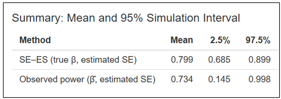
To visualize the contrast, I have created a companion Shiny app. It lets you vary sample size (n), target/true power, and α, then: (1) runs Monte Carlo replications of Y ~ 1 + βX; (2) plots side‑by‑side histograms of retrospective power for SE–ES and Observed Power; and (3) reports the Mean and the 95% simulation interval (the central 2.5%–97.5% range of simulated power values) for each method. Power is calculated under two‑tailed testing.
What you should see: the Observed Power histogram tracks the significance test—mass near 0 when results are null, near 1 when they are significant—because it is just a re‑expression of the t statistic. Further, the wide range of estimates makes it unusable even if its biasedness did not. The SE–ES histogram, in contrast, concentrates near the design’s target power and tightens as sample size grows.
To use the app, click here. Input the respective values in the Shiny app’s sidebar panel. The panel below provides an example with sample size set equal to 100; true power equal to 80% (for two-sided significance), alpha equal to 5%, and sets the number of simulations = 1000 and the random seed equal to 123.

Once you have entered your input values, click “Run simulation”. Two histograms will appear. The histogram to the left reports the distribution of estimated power values using the SE-ES method. The histogram to the right reports the same using Observed Power. The vertical dotted line indicates true power.
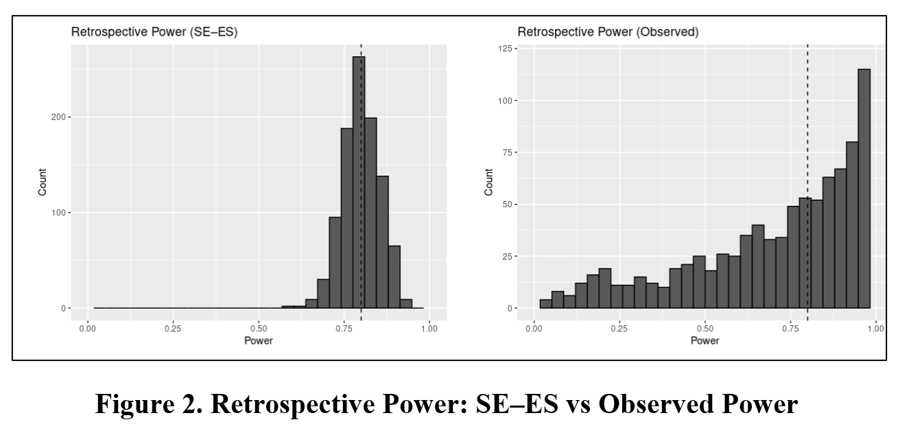
Immediately below this figure, the Shiny app produces a table that reports the mean and 95% estimation interval of estimated powers for the SE-ES and Observed Power methods. For this example, with the true power = 80%, the Observed Power distribution is left skewed, biased downwards (mean = 73.4%) with a 95% estimation interval of (14.5%, 99.8%). In contrast, the SE-ES distribution is approximately symmetric, approximately centered around the true of 80%, with a 95% estimation interval of (68.5%, 89.9%).
The reader is encouraged to try out different target power values and, most importantly, sample sizes. What you should see is that the SE-ES method works well at every true power value, but, in this context, it becomes less serviceable for sample sizes below 30.
E. Bottom line—and an easy calculator you can use now
Power estimation is useful for before estimation, for planning. But it is also useful after estimation, as an interpretative tool. Furthermore, it is easy to calculate. For readers interested in calculating retrospective power for their own research, Thomas Logchies and I have created an online calculator that is easy to use: click here. There you can enter α, degrees of freedom, an estimated standard error, and a hypothesized effect size to obtain SE–ES retrospective power for your estimate. Give it a go!
NOTE: Bob Reed is Professor of Economics and the Director of UCMeta at the University of Canterbury. He can be reached at bob.reed@canterbury.ac.nz.
References
Cumming, G. (2014). The new statistics: Why and how. Psychological Science, 25(1), 7–29. https://doi.org/10.1177/0956797613504966
Doyle, M.-A., & Feeney, L. (2021). Quick guide to power calculations. https://www.povertyactionlab.org/resource/quick-guide-power-calculations
Gelman, A., & Carlin, J. (2014). Beyond power calculations: Assessing type S (sign) and type M (magnitude) errors. Perspectives on Psychological Science, 9(6), 641–651. https://sites.stat.columbia.edu/gelman/research/published/retropower_final.pdf
Goodman, S. N., & Berlin, J. A. (1994). The use of predicted confidence intervals when planning experiments and the misuse of power when interpreting results. Annals of Internal Medicine, 121(3), 200–206. https://doi.org/10.7326/0003-4819-121-3-199408010-00008
Hoenig, J. M., & Heisey, D. M. (2001). The abuse of power: The pervasive fallacy of power calculations for data analysis. The American Statistician, 55(1), 19–24. https://doi.org/10.1198/000313001300339897
Maxwell, S. E., Kelley, K., & Rausch, J. R. (2008). Sample size planning for statistical power and accuracy in parameter estimation. Annual Review of Psychology, 59(1), 537–563. https://doi.org/10.1146/annurev.psych.59.103006.093735
McKenzie, D., & Ozier, O. (2019, May 16). Why ex-post power using estimated effect sizes is bad, but an ex-post MDE is not. Development Impact (World Bank Blog). https://blogs.worldbank.org/en/impactevaluations/why-ex-post-power-using-estimated-effect-sizes-bad-ex-post-mde-not
Tian, J., Coupé, T., Khatua, S., Reed, W. R., & Wood, B. D. (2025). Power to the researchers: Calculating power after estimation. Review of Development Economics, 29(1), 324-358. https://doi.org/10.1111/rode.13130
AoI*: “Introducing Synchronous Robustness Reports” by Bartos et al. (2025)
[*AoI = “Articles of Interest” is a feature of TRN where we report abstracts of recent research related to replication and research integrity.]
NOTE: The article is behind a firewall.
ABSTRACT (taken from the article)
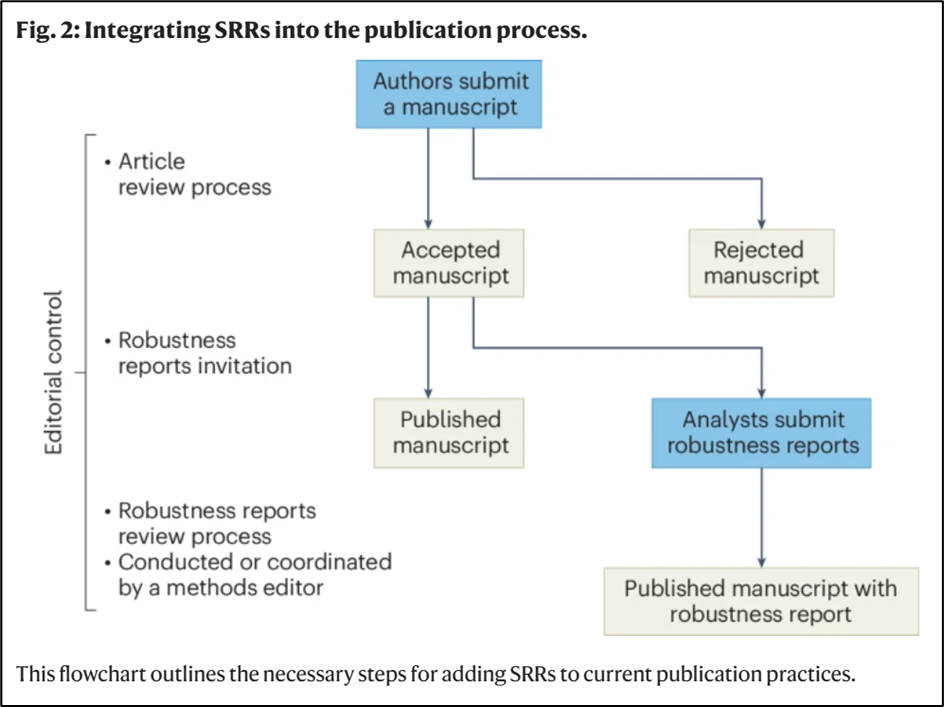
“Most empirical research articles feature a single primary analysis that is conducted by the authors. However, different analysis teams usually adopt different analytical approaches and frequently reach varied conclusions. We propose synchronous robustness reports [SRRs] — brief reports that summarize the results of alternative analyses by independent experts — to strengthen the credibility of science.”
“To integrate SRRs seamlessly into the publication process, we suggest the framework outlined as a flowchart in Fig. 2. As the flowchart shows, the SRRs form a natural extension to the standard review process.”
REFERENCE
AoI*: “The Sources of Researcher Variation in Economics” by Huntington-Klein et al. (2025)
[*AoI = “Articles of Interest” is a feature of TRN where we report abstracts of recent research related to replication and research integrity.]
ABSTRACT (taken from the article)
“We use a rigorous three-stage many-analysts design to assess how different researcher decisions—specifically data cleaning, research design, and the interpretation of a policy question—affect the variation in estimated treatment effects.”
“A total of 146 research teams each completed the same causal inference task three times each: first with few constraints, then using a shared research design, and finally with pre-cleaned data in addition to a specified design.”
“We find that even when analyzing the same data, teams reach different conclusions. In the first stage, the interquartile range (IQR) of the reported policy effect was 3.1 percentage points, with substantial outliers.”
“Surprisingly, the second stage, which restricted research design choices, exhibited slightly higher IQR (4.0 percentage points), largely attributable to imperfect adherence to the prescribed protocol. By contrast, the final stage, featuring standardized data cleaning, narrowed variation in estimated effects, achieving an IQR of 2.4 percentage points.”
“Reported sample sizes also displayed significant convergence under more restrictive conditions, with the IQR dropping from 295,187 in the first stage to 29,144 in the second, and effectively zero by the third.”
“Our findings underscore the critical importance of data cleaning in shaping applied microeconomic results and highlight avenues for future replication efforts.”
REFERENCE
AoI*: “Decisions, Decisions, Decisions: An Ethnographic Study of Researcher Discretion in Practice” by van Drimmelen et al. (2024)
[*AoI = “Articles of Interest” is a feature of TRN where we report abstracts of recent research related to replication and research integrity.]
ABSTRACT (taken from the article)
“This paper is a study of the decisions that researchers take during the execution of a research plan: their researcher discretion. Flexible research methods are generally seen as undesirable, and many methodologists urge to eliminate these so-called ‘researcher degrees of freedom’ from the research practice. However, what this looks like in practice is unclear.”
“Based on twelve months of ethnographic fieldwork in two end-of-life research groups in which we observed research practice, conducted interviews, and collected documents, we explore when researchers are required to make decisions, and what these decisions entail.”
“Our ethnographic study of research practice suggests that researcher discretion is an integral and inevitable aspect of research practice, as many elements of a research protocol will either need to be further operationalised or adapted during its execution. Moreover, it may be difficult for researchers to identify their own discretion, limiting their effectivity in transparency.”
REFERENCE
AoI*: “Open minds, tied hands: Awareness, behavior, and reasoning on open science and irresponsible research behavior” by Wiradhany et al. (2025)
[*AoI = “Articles of Interest” is a feature of TRN where we report abstracts of recent research related to replication and research integrity.]
ABSTRACT (taken from the article)
“Knowledge on Open Science Practices (OSP) has been promoted through responsible conduct of research training and the development of open science infrastructure to combat Irresponsible Research Behavior (IRB). Yet, there is limited evidence for the efficacy of OSP in minimizing IRB.”
“We asked N=778 participants to fill in questionnaires that contain OSP and ethical reasoning vignettes, and report self-admission rates of IRB and personality traits. We found that against our initial prediction, even though OSP was negatively correlated with IRB, this correlation was very weak, and upon controlling for individual differences factors, OSP neither predicted IRB nor was this relationship moderated by ethical reasoning.”
“On the other hand, individual differences factors, namely dark personality triad, and conscientiousness and openness, contributed more to IRB than OSP knowledge.”
“Our findings suggest that OSP knowledge needs to be complemented by the development of ethical virtues to encounter IRBs more effectively.”
REFERENCE
RÖSELER: Replication Research Symposium and Journal
Efforts to teach, collect, curate, and guide replication research are culminating in the new diamond open access journal Replication Research, which will launch in late 2025. The Framework for Open and Reproducible Research Training (FORRT; forrt.org) and the Münster Center for Open Science have spearheaded several initiatives to bolster replication research across various disciplines. From May 14-16, 2025, we are excited to invite researchers to join us in Münster, as well as online, for the Replication Research Symposium. This event will mark a significant step toward the launch of our interdisciplinary journal dedicated to reproductions, replications, and discussions on the methodologies involved. But let’s start from the beginning: What is going on at FORRT?
Finding and exploring replications: FORRT Replication Database (FReD) includes hundreds of replication studies and thousands of replication findings – which we define as tests of previously established claims using different data. Researchers can use the Annotator to have their reference lists auto-checked to see whether they cited original studies that have been replicated. With the Explorer, they get an overview of all studies and can analyze replication rates across different success criteria or moderator variables.
Meta-analyzing replication outcomes: To increase the accessibility of the database, we created the FReD R-package with which researchers can run their own analyses or run the ShinyApps locally. In a vignette, we outline different replication success criteria and show how this choice can affect the overall replication success rate.
Teaching replications: One of FORRT’s core ideas is to support researchers from all fields to learn about openness and reproducibility. Among numerous projects, we clarified terminology (Glossary of Open Science Terms), produced educational materials such as an educationally-driven review paper on the transformative impact of the replication crisis, syllabus and slides with lecture and pedagogical notes (see Educational toolkit), and curated resources. We are also now working together with experts from economics, psychology, medicine, and other fields to create an interdisciplinary guide to carrying out replications and reproductions.
Publishing replication studies and discussing standards across fields: We are currently developing the journal Replication Research, a diamond open-access outlet for replication and reproduction studies and discussions about the respective methods. There will be reproducibility checks for all published studies and standardized machine-readable templates that authors are encouraged to use. We are currently building the journal with a network of 20 experts from different fields. From February until April, we are organizing the Road to Replication Research via Zoom. This online discussion series is centered around different aspects of open and responsible scientific publishing and is open to anybody who wants to join the conversation, so that the journal is maximally open from the start. Finally, at the Replication Research Symposium, participants and experts from diverse fields such as psychology, economics, biology, medicine, marketing, meta-science, library science, humanities, and others will convene to discuss the significance and methodology of conducting replication and reproduction studies over three days in May 2025. This symposium will further shape Replication Research and we invite researchers from all fields to present their replications, reproductions, or methodological discussions. The journal launch is then slated for late 2025.
For more information about Replication Research, the upcoming symposium, and the online discussion series about the creation of the journal click here.
Lukas Röseler is the managing director of the Münster Center for Open Science at the University of Münster, one of the project leads at FORRT’s Replication Hub, and will be the managing editor of Replication Research. He can be contacted at lukas.roeseler@uni-muenster.de.

ROODMAN: Appeal to Me – First Trial of a “Replication Opinion”
Posted on by replicationnetwork
Leave a Comment
[This blog is a repost of a blog that first appeared at davidroodman.com. It is republished here with permission from the author.]
My employer, Open Philanthropy, strives to make grants in light of evidence. Of course, many uncertainties in our decision-making are irreducible. No amount of thumbing through peer-reviewed journals will tell us how great a threat AI will pose decades hence, or whether a group we fund will get a vaccine to market or a bill to the governor’s desk. But we have checked journals for insight into many topics, such as the odds of a grid-destabilizing geomagnetic storm, and how much building new schools boosts what kids earn when they grow up.
When we draw on research, we vet it in rare depth (as does GiveWell, from which we spun off). I have sometimes spent months replicating and reanalyzing a key study—checking for bugs in the computer code, thinking about how I would run the numbers differently and how I would interpret the results. This interface between research and practice might seem like a picture of harmony, since researchers want their work to guide decision-making for the public good and decision-makers like Open Philanthropy want to receive such guidance.
Yet I have come to see how cultural misunderstandings prevail at this interface. From my side, there are two problems. First, about half the time I reanalyze a study, I find that there are important bugs in the code, or that adding more data makes the mathematical finding go away, or that there’s a compelling alternative explanation for the results. (Caveat: most of my experience is with non-randomized studies.)
Second, when I send my critical findings to the journal that peer-reviewed and published the original research, the editors usually don’t seem interested (recent exception).
Seeing the ivory tower as a bastion of truth-seeking, I used to be surprised. I understand now that, because of how the academy works, in particular, because of how the individuals within academia respond to incentives beyond their control, we consumers of research are sometimes more truth-seeking than the producers.
Last fall I read a tiny illustration of the second problem, and it inspired me to try something new. Dartmouth economist Paul Novosad tweeted his pique with economics journals over how they handle challenges to published papers:
As you might glean from the truncated screenshots, the starting point for debate is a paper published in 2019. It finds that U.S. immigration judges were less likely to grant asylum on warmer days. For each 10°F the temperature went up, the chance of winning asylum went down 1 percentage point.
The critique was written by another academic. It fixes errors in the original paper, expands the data set, and finds no such link from heat to grace. In the rejoinder, the original authors acknowledge errors but say their conclusion stands. “AEJ” (American Economic Journal: Applied Economics) published all three articles in the debate. As you can see, the dueling abstracts confused even an expert.
So I appointed myself judge in the case. Which I’ve never seen anyone do before, at least not so formally. I did my best to hear out both sides (though the “hearing” was reading), then identify and probe key points of disagreement. I figured my take would be more independent and credible than anything either party to the debate could write. I hoped to demonstrate and think about how academia sometimes struggles to serve the cause of truth-seeking. And I could experiment with this new form as one way to improve matters.
I just filed my opinion, which is to say, the Institute for Replication has posted it. (Open Philanthropy partly funds them.) My colleague Matt Clancy has pioneered living literature reviews; he suggested that I make this opinion a living document as well. If either party to the debate, or anyone else, changes my mind about anything in the opinion, I will revise it while preserving the history.
Verdict
My conclusion was more one-sided than I had expected. I came down in favor of the commenter. The authors of the original paper defend their finding by arguing that in retrospect they should have excluded the quarter of their sample consisting of asylum applications filed by people from China. Yes, they concede, correcting the errors mostly erases their original finding. But it reappears after Chinese are excluded.
This argument did not persuade me. True, during the period of this study, 2000–04, most Chinese asylum-seekers applied under a special U.S. law meant to give safe harbor to women fearing forced sterilization and abortion in their home country.
The authors seem to argue that because grounds for asylum were more demonstrable in these cases—anyone could read about the draconian enforcement of China’s one-child policy—immigration judges effectively lacked much discretion. And if outdoor temperature couldn’t meaningfully affect their decisions, the cases were best dropped from a study of precisely that connection.
But this premise is flatly contradicted by a study the authors cite called “Refugee Roulette.” In the study, Figure 6 shows that judges differed widely in how often they granted asylum to Chinese applicants. One did so less than 5% of the time, another more than 90%, and the rest were spread evenly between. (For a more thorough discussion, read sections 4.4 and 6.1 of my opinion.)
Thus while I do not dispute that there is a correlation between temperature and asylum grants in a particular subset of the data, I think it is best explained by p-hacking or some other form of “filtration,” in which, consciously or not, researchers gravitate toward results that happen to look statistically significant. (In fairness, they know that peer reviewers, editors, and readers gravitate to the same sorts of results, and getting a paper into a good journal can make a career.)
The nature of the defense raises a question about how the journal handled the dispute. It published the original authors’ rejoinder as a Correction. Yet, while one might agree that it is better to exclude Chinese from the analysis, I think their inclusion in the original was not an error, and therefore their exclusion is not a correction. Thus, one way the journal might have headed off Novosad’s befuddlement would have been by insisting that Corrections only make corrections.
What’s wrong with this picture?
To recap:
– Two economists performed a quantitative analysis of a clever, novel question.
– It underwent peer review.
– It was published in one of the top journals in economics. Its data and computer code were posted online, per the journal’s policy
– Another researcher promptly responded that the analysis contains errors (such as computing average daytime temperature with respect to Greenwich time rather than local time), and that it could have been done on a much larger data set (for 1990 to ~2019 instead of 2000–04). These changes make the headline findings go away.
– After behind-the-scenes back and forth among the disputants and editors, the journal published the comment and rejoinder.
– These new articles confused even an expert.
– An outsider (me) delved into the debate and found that it’s actually a pretty easy call.
If you score the journal on whether it successfully illuminated its readership as to the truth, then I think it is kind of 0 for 2.
[Update: I submitted the opinion to the journal, which promptly rejected it. I understand that the submission was an odd duck. But if I’m being harsh I can raise the count to 0 for 3.]
That said, AEJ Applied did support dialogue between economists that eventually brought the truth out. In particular, by requiring public posting of data and code (an area where this journal and its siblings have been pioneers), it facilitated rapid scrutiny.
Still, it bears emphasizing: For quality assurance, the data sharing was much more valuable than the peer review. And, whether for lack of time or reluctance to take sides, the journal’s handling of the dispute obscured the truth.
My purpose in examining this example is not to call down a thunderbolt on anyone, from the Olympian heights of a funding body. It is rather to use a concrete story to illustrate the larger patterns I mentioned earlier.
Despite having undergone peer review, many published studies in the social sciences and epidemiology do not withstand close scrutiny. When they are challenged, journal editors have a hard time managing the debate in a way that produces more light than heat.
I have critiqued papers about the impact of foreign aid, microcredit, foreign aid, deworming, malaria eradication, foreign aid, geomagnetic storm risk, incarceration, schooling, more schooling, broadband, foreign aid, malnutrition, ….
Many of those critiques I have submitted to journals, typically only to receive polite rejections. I obviously lack objectivity. But it has struck me as strange that, in these instances, we on the outside of academia seem more concerned about getting to the truth than those on the inside. Sometimes I’ve wished I could appeal to an independent authority to review a case and either validate my take or put me in my place.
That yearning is what primed me to respond to Novosad’s tweet by donning the robe of a judge myself. (I passed on the wig.)
I’ve never edited a journal, but I’ve talked to people who have, and I have some idea of what is going on. Editors juggle many considerations besides squeezing maximum truth juice out of any particular study. Fully grasping a replication debate takes work—imagine the parties lobbing 25-page missives at each other, dense with equations, tables, and graphs—and editors are busy.
Published comments don’t get cited much anyway, and editors keep an eye on how much their journals get cited. They may also weigh the personal costs for the people whose reputations are at stake. Many journals, especially those published by professional associations, want to be open to all comers—to be the moderator, not the panelist, the platform, not the content provider.
The job they set for themselves is not quite to assess the reliability of any given study (a tall order) but to certify that each article meets a minimum standard, to support the collective dialogue through which humanity seeks scientific truth.
Then, too, I think journal editors often care a lot about whether a paper makes a “contribution” such as a novel question, data source, or analytical method. Closer to home, junior editors may think twice before welcoming criticism that could harm the reputation of their journal or ruffle the feathers of more powerful members of their flock. Senior editors may have gotten where they are by thinking in the same, savvy way.
Modern science is the best system ever developed for pursuing truth. But it is still populated by human beings (for how much longer?) whose cognitive wiring makes the process uncomfortable and imperfect. Humans are tribal creatures—not as wired for selflessness as your average ant, but more apt to go to war than an eel or an eagle.
Among the bits of psychological glue that bind us are shared ideas about “is” and “ought.” Imperialists and evangelists have long influenced shared ideas in order to expand and solidify the groups over which they hold sway. The links between belief, belonging, and power are why the notion that evidence trumps belief was so revolutionary when the Roman church sent Galileo to his death, and why the idea, despite making modernity possible, remains discomfiting to this day.
The inefficiency in pursuing truth has real costs for society. Some social science research influences decisions by private philanthropies and public agencies, decisions whose stakes can be measured in human lives, or in the millions, billions, even trillions of dollars. Yet individual studies receive perhaps hundreds of dollars worth of time in peer review, and that within a system in which getting each paper as close as possible to the truth is one of several competing priorities.
Making science work better is the stuff of metascience, an area in which Open Philanthropy makes grants. It’s a big topic. Here, I’ll merely toss out the idea that if these new-fangled replication opinions were regularly produced, they could somewhat mitigate the structural deprecation of truth-seeking.
On the demand side—among decision-makers using research—replication opinions could improve the vetting of disputed studies, while efficiently targeting the ones that matter most. (Related idea here.)
On the supply side, a heightened awareness that an “appeals court” could upstage journals in a role laypeople and policymakers expect them to fill—performing quality assurance on what they publish—could stimulate the journals to handle replication debates in a way that better serves their readers and society.
Reflections on writing the replication opinion
Writing a novel piece led me to novel questions. To prepare for writing my opinion, I read about how judges write theirs. Judicial opinions usually have a few standard sections. They review the history of the case (what happened to bring it about, what motions were filed); list agreed facts; frame the question to be decided; enunciate some standard that a party has to meet, perhaps handed down by the Supreme Court; and then bring the facts to the standard to reach a decision.
Could I follow that outline? Reviewing the case history was easy enough. I had the papers and could inventory their technical points. The data and computer code behind the papers are on the web, so I could rerun the code and stipulate facts such as that a particular statistical procedure applied to a particular data set generates a particular output.
Figuring out what I was trying to judge was harder. Surely it was not whether, for all people, places, and times, heat makes us less gracious. Nor should I try to decide that question even in the study’s context, which was U.S. asylum cases decided between 2000 and 2004.
Truth in the social sciences is rarely absolute. We use statistics precisely because we know that there is noise in every measurement, uncertainty in every finding. In addition, by Bayes’ Rule, the conclusions we draw from any one piece of evidence depend on the prior knowledge we bring to it, which is shaped by other evidence.
Someone who has read 10 ironclad articles on how temperature affects asylum decisions should hardly be moved by one more. Yet I think those 10 other studies, if they existed, would lie beyond the scope of this case.
That means that my replication opinion is not about the effects of temperature on behavior in any setting. It’s more meta than that. It’s about how much this new paper should shift or strengthen one’s views on the question.
After reflecting on these complications, here is what I decided to decide: to the extent that a reasonable observer updated their priors after reading the original paper, how much should the subsequent debate reverse or strengthen that update?
My judgment need not have been binary. Unlike a jury burdened with deciding guilt or innocence, a replication opinion can come down in the middle, again by Bayes’ Rule. Sometimes there is more than one reasonable way to run the numbers and more than one reasonable way to interpret the results.
I sought rubrics through which to organize my discussion—both to discipline my own reasoning and to set precedents, should I or anyone else do this again. I borrowed a typology developed by former colleague Michael Clemens of the varieties of replication and robustness testing, as well as a typology of statistical issues from Shadish, Cook, and Campbell.
And I made a list of study traits that we can expect to be associated, on average, with publication bias and other kinds of result filtration. For example, there is evidence that in top journals, statistical results from junior economists, who are running the publish-or-perish gauntlet toward tenure, are more likely to report results that just clear conventional thresholds for statistical significance. That is consistent with the theory that the researchers on whom the system’s perverse incentives impinge most strongly are most apt to run the numbers several ways and emphasize the “significant” runs in their write-ups.
One tricky issue was how much I should analyze the data myself. The upside could be more insight. The downside could be a loss of (perceived) objectivity if the self-appointed referee starts playing the game. Wisely or not, I gave myself some leeway here. Surely real judges also rely on their knowledge about the world, not just what the parties submit as evidence.
For example, in addition to its analysis of asylum decisions, the original paper checks whether the California parole board was less likely to grant parole on warmer days in 2012–15. Partly because the critical comment did not engage with this side-analysis, I revisited it myself. I transferred it to the next quadrennium, 2016–19, while changing the original computer code as little as possible. (Here, too, the apparent impact of temperature went away.)
Closing statement
The stakes in this case are probably low. While the question of how temperature affects human decision-making links broadly to climate change, and the arbitrariness of the American immigration system is a serious concern, I would be surprised if any important policy decision in the next few years turns on this research.
But the case illustrates a much larger problem. Some studies do influence important decisions. That they have been peer-reviewed should hardly reassure. Judicious post-publication review of important studies, perhaps including “replication opinions,” can give decision-makers with real dollars and real livelihoods on the line a clearer sense of what the data do and do not tell us.
Unfortunately, powerful incentives within academia, rooted in human nature, have generally discouraged such Socratic inquiry.
I like to think of myself as judicious. As to whether I’ve lived up to my self-image in this case, I will let you be the judge. At any rate, I figure that in the face of hard problems, it is good to try new things. We will see if this experiment is replicated, and if that does much good.
David Roodman is Senior Advisor at Open Philanthropy. He can be contacted at david@davidroodman.com
Category: GUEST BLOGS Tags: Academic incentives, Comments, economics, Evidence-based policy, Journal policy, Meta-Science, Open Philanthropy, peer review, replications, Truth-seeking