[From the blog “Where Do Non-Significant Results in Meta-Analysis Come From?” by Ulrich Schimmack, posted at Replicability-Index]
“It is well known that focal hypothesis tests in psychology journals nearly always reject the null-hypothesis … However, meta-analyses often contain a fairly large number of non-significant results. … Here I used the extremely well-done meta-analysis of money priming studies to explore this issue …”
“Out of 282 tests, only 116 (41%) are significant. This finding is surprising, given the typical discovery rates over 90% in psychology journals.”
“Publication bias implies that studies with non-significant results end up in the proverbial file-drawer. …The money-priming meta-analysis included 113 unpublished studies. … The observed discovery rate is slightly lower than for the full set of studies, 29%.”
“The complementary finding for published studies … is that the observed discovery rate increases, 49%…”
“In response to concerns about publication bias and questionable research practices, psychology journals have become more willing to publish null-results. An emerging format are pre-registered replication studies with the explicit aim of probing the credibility of published results. The money priming meta-analysis included 47 independent replication studies. … independent replication studies had a very low observed discovery rate, 4%…”
“Removing independent replication studies from the set of published studies further increases the observed discovery rate, 66%.”
“After a (true or false) effect has been established in the literature, follow up studies often examine boundary conditions and moderators of an effect. Evidence for moderation is typically demonstrated with interaction effects that are sometimes followed by contrast analysis for different groups. …”
“…meta-analysts often split the sample and treat different subgroups as independent samples. This can produce a large number of non-significant results because a moderator analysis allows for the fact that the effect emerged only in one group. The resulting non-significant results may provide false evidence of honest reporting of results because bias tests rely on the focal moderator effect to examine publication bias.”
“The analysis of the published main effect shows a dramatically different pattern. The observed discovery rate increased to 56/67 = 84%.”
“I also examined more closely the … non-significant results in this set of studies.”
“… none of the … studies with non-significant results in the meta-analysis that were published in a journal reported that money priming had no effect on a dependent variable. All articles reported some significant results as the key finding. This further confirms how dramatically publication bias distorts the evidence reported in psychology journals.”
“In this blog post, I examined the discrepancy between null-results in journal articles and in meta-analysis, using a meta-analysis of money priming. While the meta-analysis suggested that publication bias is relatively modest, published articles showed clear evidence of publication bias …”
“Three factors contributed to this discrepancy: (a) the inclusion of unpublished studies, (b) independent replication studies, and (c) the coding of interaction effects as separate effects for subgroups rather than coding the main effect.”
In Frequentist statistical inference, the p-value is used as a measure of how incompatible the data are with the null hypothesis. When the null hypothesis is fixed at a point, the test statistic reports a distance from the sample statistic to this point. A low (high) p-value means that this distance is large (small), relative to the sampling variability. Hence, the p-value also reports this distance, but in a different scale, namely the scale of probability.
In a recent article published in Econometrics (“Interval-Based Hypothesis Testing and Its Applications to Economics and Finance”), we highlight the problems with the p-value criterion in concert with point null hypotheses. We propose that researchers move to interval-based hypothesis testing instead. While such a proposal is not new (Hodges and Lehmann, 1954) and such tests are being used in biostatistics and psychology (Welleck, 2010), it is virtually unknown to economics and business disciplines. In what follows, we highlight problems with the p-value criterion and show how they can be overcome by adopting interval-based hypothesis testing.
The first problem concerns economic significance; namely, whether the distance between the sample statistic and the point under the null has any economic importance. The p-value has nothing to say about this: it only reports whether the distance is large relative to the variability — not the relevance of the distance. It is certainly possible to have statistically significant results that are economically or operationally meaningless.
The second problem is that the implied critical value of the test changes very little with sample size, while the test statistic generally increases with sample size. This is because the sampling distribution does not change, or does not change much. Stated differently, the distribution from which one obtains the critical value is (nearly) the same, regardless of how large or small sample size (or statistical power) is.
And last but not least, since the population parameter can never be exactly equal to the null value under the point-null hypothesis, the sampling distribution under the null hypothesis is never realized or observed in reality. As a result, when a researcher calculates a t-statistic, it is almost certain that she obtains the value from a distribution under the alternative (a non-central t-distribution), and not from the distribution under the null (a central t-distribution). This can cause the critical value from the central distribution to be misleading, especially when the sample size is large.
Consider a simple t-test for H0:θ=0, where θ represents the population mean. Assuming a random sample from a normal distribution with unknown standard deviation σ, the test statistic is t = n0.5Xbar/σ where σ denotes the sample standard deviation. The test statistic follows a Student-t distribution with (n-1) degrees of freedom and non-centrality parameter λ=n0.5θ/σ, denoted as t(n-1; λ). Under H0, the t-statistic follows a central t-distribution with λ=0.
In reality, the value of θ cannot exactly and literally be 0. As Delong and Lang (1992) point out, “almost all tested null hypothesis in economics are false”. The consequence is that, with observational data, a t-statistic is (almost) always generated from a non-central t-distribution, not from a central one.
Suppose the value of θ was in fact 0.1 and that this value implies no economic or practical importance. That is, H0 practically holds. Let us assume for simplicity that σ=1. When n = 10, the t-statistic is in fact generated from t(9; λ=0.316), not from t(9; λ=0). When the sample size is small — for example, 10 — the two distributions are very close, so the p-value can be a reasonable indicator for the evidence against H0. When the sample size is larger, say 1000, the t-statistic is generated from t(999; λ=3.16). When it is 5000, it is generated from t(4999; λ=7.07). Under the point-null hypothesis, the distribution is fixed at t(n-1; λ=0). At this large sample size, every t-statistic is larger than the critical value at a conventional level; and every p-value is virtually equal to 0. Hence, although economically insignificant, a sample estimate of θ=0.1 will be statistically significant with a large t-statistic and a near-zero p-value.
This situation is illustrated in Figure 1, where the black curve plots the central t-distribution; and red and blue curves show non-central distributions respectively for λ=0.316 and λ=7.07. The blue curve is an essentially a normal distribution, but for the purpose of illustration, we maintain it as a t-distribution with λ > 0. The point-null hypothesis fixes the sampling distribution at the black curve which is t(n-1; λ=0), so the 5% critical value does not change (no more than 1.645) regardless of sample size.
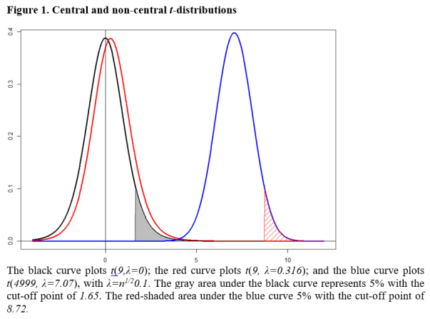
The consequence is that, when the value of λ is as large as 7.07 with a large sample size, the null hypothesis is almost always rejected with the p-value virtually 0, even though θ=0.1 is economically negligible. The problem may not be serious when the sample size is small, but it is when the sample size is large. We now show how adopting an interval hypothesis allows one to overcome this problem.
Consider H0: 0 < θ ≤ 0.5 against H1: θ > 0.5. Let the value of θ = 0.5 be the minimum value of economic importance. Under the null hypothesis, the mean is economically negligible or practically no different from 0; while it makes a difference economically under H1. This class of interval-based tests is called minimum-effect tests.
The decision rule is to reject H0 at the 5% level if the t-statistic is greater than the critical value from t(n-1, λ=n1/20.5) distribution. That is, the critical value increases with the sample size. If this distribution were the blue curve in Figure 1, the corresponding 5% critical value would be 8.72, indicated by the cut-off value corresponding to the red-shaded area.
In conducting an interval-based test, choosing the interval of economic significance is crucial for the credibility of the test. It should be set by the researcher, based on economic analysis or value judgment, desirably with a consensus from other researchers and ideally before she observes the data.
With such an interval hypothesis, a clear statement is made on the economic significance of the parameter and is taken into account for decision-making. In addition, the critical value and the sampling distribution of the test change with sample size; and the p-value is not necessarily a decreasing function of sample size.
As a practical illustration, we analyze the Halloween effect (Bouman and Jacobsen, 2002), where it is claimed that stock returns are consistently higher from the period of November to April. They fit a simple regression model of the form
Rt = γ0 + γ1 Dt + ut,
where Rt is stock return in percentage and Dt is a dummy variable which takes 1 from November to April; and 0 otherwise.
Using monthly data for a large number of stock markets around the world, Bouman and Jacobsen (2002; Table 1) report positive and statistically significant values of γ1. For the U.S. market using 344 monthly observations, they report that the estimated value of γ1 is 0.96 with a t-statistic of 1.95.
Using daily data from 1950 to 2016 (16,819 observations), we replicate their results with an estimated value of γ1=0.05 and a t-statistic of 3.44. For the point-null hypothesis H0: γ1 = 0; H1: γ1 > 0, we reject H0 at the 5% level of significance for both monthly and daily data, with p-values of 0.026 and 0.0003 respectively. The Halloween effect is statistically clear and strong, especially when the sample size is larger.
Now we conduct minimum-effect tests. We assume that the stock return should be at least 1% higher per month during the period of November to April to be considered economically significance. This value is conservative considering trading costs and the volatility of the market.
The corresponding null and alternative hypotheses are H0: 0 < γ1 ≤ 1; H1: γ1 > 1. The 5% critical value of this test is 3.66 obtained from t(342, λ=2.06). On a daily basis, it is equivalent to H0: 0 < γ1 ≤ 0.05; H1: γ1 > 0.05, assuming 20 trading days per month. The 5% critical value of this test is 5.28 obtained from t(16,817, λ=3.60). For both cases, the null hypothesis of no economic significance cannot be rejected at the 5% level of significance. That is, the Halloween effect is found to be economically negligible with interval-based hypothesis testing.
In Figure 2, we present the Box-Whisker plot of the daily returns against D. It appears that there are a lot more outliers during the non-Halloween period, but the median and the quartile values are nearly identical for the two periods.
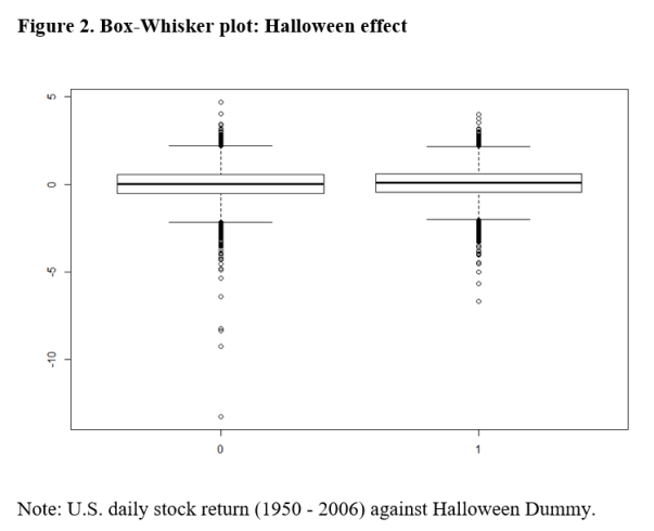
This plot provides further evidence that the Halloween effect is negligible, apart from these outliers. It is likely that the effect size estimates of the above Halloween regressions are over-stated by ignoring these outliers. This application highlights the problems of the point-null hypothesis and demonstrates how interval hypothesis testing can overcome them.
As Rao and Lovric (2016) argue, the paradigm of point-null hypothesis testing is no longer viable in the era of big data. Now is the time to adopt a new paradigm for statistical decision-making. In our article, we demonstrate that testing for an interval-null hypothesis can be a way forward.
Jae (Paul) Kim is a Professor of Finance in the Department of Finance at La Trobe University. Andrew Robinson is Director of the Centre of Excellence for Biosecurity Risk Analysis and Associate Professor in the School of Mathematics and Statistics, both at the University of Melbourne. Comments and/or questions about this blog can be directed to Professor Kim at J.Kim@latrobe.edu.au.
References
Bouman, S. Jacobsen, B. 2002. The Halloween Indicator, “Sell in May and Go Away”: Another Puzzle, American Economic Review, 92(5), 1618-1635.
DeLong, J.B. and K. Lang, 1992, Are All Economic Hypotheses False? Journal of Political Economy, Vol. 100, No. 6, pp. 1257-72.
Hodges, J. L. Jr. and E.L. Lehmann 1954, Testing the Approximate Validity of Statistical Hypotheses, Journal of the Royal Statistical Society, Series B (Methodological), Vol. 16, No. 2, pp. 261–268.
Rao, C. R. and Lovric, M. M., 2016, Testing Point Null Hypothesis of a Normal Mean and the Truth: 21st Century Perspective, Journal of Modern Applied Statistical Methods, 15 (2), 2–21.
Wellek, S., 2010, Testing Statistical Hypotheses of Equivalence and Noninferiority, 2nd edition, CRC Press, New York.
[From the article “Reproducibility trial publishes two conclusions for one paper” by David Adam, published in Nature]
“How deeply an anaesthetist should sedate an elderly person when they have surgery is a controversial issue, because some studies link stronger doses of anaesthetic with earlier deaths. So it should reassure clinicians to see a study in the British Journal of Anaesthesia that investigates and rules out such a link…”
“Another paper in the journal analyses the same results and reaches a different conclusion about death rates. It says the trial didn’t include enough patients to reach that conclusion — or any conclusion — on mortality.”
“The opposing takes on the mortality link — a secondary conclusion of the study — are the result of an unusual peer-review experiment at the journal to tackle reproducibility of results in the field.”
“…for some papers, the British Journal of Anaesthesia is now asking an independent expert to write their own discussion of the study.”
“Unlike conventional peer reviewers, they look only at the methods and results sections and are blinded to the paper’s conclusions. The two discussions sections are published together, with similarities and differences highlighted.”
“At present, critiques of papers in the journal can appear weeks or months after publication, as guest editorials for example. By publishing the independent discussion at the same time as the peer-reviewed original, the journal hopes to accelerate the self-correcting nature of the literature.”
[From the article “Pre-results review reaches the (economic) lab: Experimental Economics follows the Journal of Development Economics in piloting pre-results review”, an interview with Irenaeus Wolff, published at www.bitss.org. The following are excerpts from that interview.]
“In its April 2019 issue, the journal Experimental Economics issued a Call for Submissions for a virtual Symposium of 5-7 papers to be published under “pre-results review”. BITSS talked to Irenaeus Wolff of University of Konstanz, who along with Urs Fischbacher is a guest editor for the Symposium.”
“2. Is your main concern publication bias?”
“Yes…”
“6. What do you hope that pre-results review will achieve in your discipline?”
“First, we hope to improve the validity of research. If there is some idea that many people think is true even though it is not, then it is tremendously important that null-results get out.”
“Second, think of the case that some researcher asks an important question that opens the door to a completely new research area. However, the researcher does not find the perfect design immediately to answer the question. … an inconclusive result could help others to design better experiments …”
“Closely related to this, null results can help refine our thinking about true relationships: if we see that in everyday life, A seems to lead to B but we cannot find it in the lab, we simply might have overlooked that A leads to B only under specific circumstances. So, seeing null results could be an important step in figuring out the true relationship between A and B.”
“7. What do you see as the main advantages of pre-results review?”
“I think they are pretty clear, and a lot has been said about them. Two things might be worth mentioning still. First, in contrast to what intuition might tell us, the required effort for the publication of a paper actually may decrease.”
“The second point concerns pre-registration. Many people seem to think that pre-registration will go a long way to solve the replication crisis. I don’t think so, and not just because people do not follow the registered protocol closely. To me, it seems pretty obvious that pre-registration does little to address the publication bias, in particular because it does not increase the incentives to complete an article after a null-result—or accept it, as an editor.”
“In that sense, I am wary that the fast spread of pre-registration might in the end block the more important step towards widespread use of results-blind review, because it might make people believe we have done enough.”
“10. In the end, what do you hope to achieve by the time the special issue is out?”
“We hope that there will be a substantial number of high-quality submissions, and that the quality of the papers that end up in the Symposium is convincing. Then, we might be able to convince the editorial board—and potentially the boards of other similar journals—that there is enough demand for such a submission option, and that this does not mean there would be a drop in paper quality.”
[From the paper “Stability of experimental results: Forecasts and evidence” by Stefano DellaVigna and Devin Pope, an NBER Working Paper]
“How robust are experimental results to changes in design? And can researchers anticipate which changes matter most? We consider a specific context, a real-effort task with multiple behavioral treatments, and examine the stability along six dimensions: (i) pure replication; (ii) demographics; (iii) geography and culture; (iv) the task; (v) the output measure; (vi) the presence of a consent form.”
“The initial task is a typing task employed in DellaVigna and Pope (2018a,b): subjects on MTurk have 10 minutes to alternatively press the `a’ and `b’ buttons on their keyboards as quickly as possible.”
“We build on this experiment by considering several design variants, covering the six dimensions above and collecting data on nearly 10,000 new MTurk subjects. In each variant we include 15 of the original treatments, following a pre-registered design.”
“Moving from one design to the next, we are interested in the stability of the findings on effort for the 15 treatments. But what is the right metric of stability? … We use rank-order correlation across the treatments as measure of stability…”
“Having identified the design changes and the measure of stability, following DellaVigna and Pope (2018b) we collect forecasts. We contact 70 behavioral experts or experts on replication, yielding 55 responses. Each expert sees a description of the task, of the design changes, and an illustration of how rank-order correlation works; whenever possible, we also provide information on the full-stability benchmark. The experts then forecast the rank-order correlation for 10 design changes.”
“… the experts have at best a mixed record in their ability to predict how much design changes affect the results. This contrasts with recent evidence that experts are able to predict quite accurately replication in pure-replication studies (Dreber et al., 2015; Camerer et al., 2016) … This confirms the anecdotal impression that design choices are a somewhat unpredictable part of the experimenter toolbox, and suggests that external validity judgments may be more tentative than we realize.”
To read the paper, click here. (NOTE: paper is behind a paywall.)
[* EiR = Econometrics in Replications, a feature of TRN that highlights useful econometrics procedures for re-analysing existing research. The material for this blog is drawn from the recent working paper “Two-way fixed effects estimators with heterogeneous treatment effects” by Clément de Chaisemartin and Xavier D’Haultfoeuille, posted at ArXiv.org]
NOTE #1: All the data and code (Stata) necessary to produce the results in the tables below are available at Harvard’s Dataverse: click here.
NOTE #2: Since this blog was written, the “breps” and “brepscluster” options have been removed from the twowayfeweights command (see below).
It is common to estimate treatment effects within a model incorporating both group and time fixed effects (think Differences-in-Differences). In a recent paper, Clément de Chaisemartin and Xavier D’Haultfoeuille (henceforth C&D) demonstrate how these models can produce unreliable estimates of average treatment effects when effects are heterogeneous across groups and time periods.
Their paper both identifies the problem and provides a solution. The purpose of this blog is to enable others to use C&D’s procedures to re-analyze published research.
In what follows, I highlight key points from their paper. Following their paper, I illustrate the problem, discuss the solution, and show how it makes a difference in replicating a key result from Gentzkow et al. (2011).
The Problem
Consider the following two-group, three-period data, where groups are designated by g = 0,1 and time periods by t = 0,1,2.
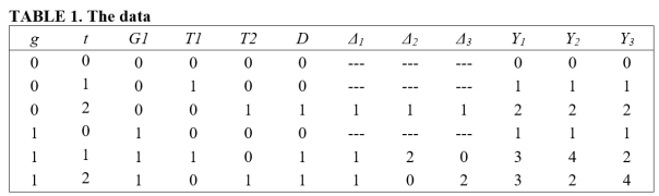
G1, T1, and T2 are dummy variables indicating whether an observation belongs to the first group, first time period, and second time period, respectively. D is a treatment indicator that takes the value 1 if the particular (g,t) cell received treatment. Note that treatment is applied to group g=0 at time t=2, and to group g=1 at times t=1,2.
Δ indicates the size of the treatment effect for treated cells (we ignore the size of the treatment effect for the untreated cells). Consider three regimes for Δ.
In the first regime (Δ1), the treatment effect is homogeneous across groups and time periods. In the second regime (Δ2), the treatment effects are heterogeneous, with the treatment effect equalling 1 for (g,t) = (0,2), and 2 and 0 for cells (g,t) = (1,1) and (g,t) = (1,2), respectively. The third regime (Δ3) is similar, except that the sizes of the treatment effects are reversed for group g=1, with treatment effects equal to 0 and 2 in time periods 1 and 2. Note that the average treatment effect for the treated (ATT) equals 1 for all three treatment regimes.
Let the outcome for each observation be determined by the following equation:
Ygt = Δgt∙Dgt + G1gt + T1gt + T2gt , g=0,1; t=0,1,2.
Suppose one estimates the following regression specification using OLS:
(1) Ygt = β0 + βfe Dgt + βG1G1gt + βT1T1gt + βT2T2gt + error.
In this specification, the treatment effect is estimated by βfe, the coefficient on the treatment dummy variable. C&D prove that βfe can be expressed as a weighted average of the individual treatment effects:
βfe = w02Δ02 + w11Δ11 + w12Δ12 ,
where w02 + w11 + w12 = 1; and Δ02 , Δ11, and Δ12 represent the treatment effects associated with the (g,t) cells (0,2), (1,2), and (1,3) for a given treatment regime.
What follows is quite surprising. C&D demonstrate that the weights need not all be positive. In fact, it can be shown in the current case that:
βfe = (½ Δ02) + Δ11 + (-½ Δ12) .
Where does the negative weight on the third treatment effect come from? βfe is the average of two difference-in-differences. The first is associated with the change in treatment for g=0 over the time periods t=1,2 (DID0). The second relates to the change in treatment for g=1 over the time periods t=0,1 (DID1). Specifically,
βfe = (DID0 + DID1)/2.
First consider DID0 = [E(Y02) – E(Y01)] -[E(Y12) – E(Y11)] = Δ02 – (Δ12 – Δ11).
The first term in brackets in DID0 measures the change in outcomes for the treatment observations associated with the first change in treatment. The second term in brackets represents the change in outcomes for the control observations over the same period. Note that both control observations receive treatment.
Ignoring time trends (as they cancel out under the common trend assumption), if treatment effects are homogeneous, the latter term, [E(Y12) – E(Y11)] = (Δ12 – Δ11), will drop out. But if the treatment effect for group g=1 is different for periods t=1,2, this term remains. Further, if the treatment effect in t=2 is sufficiently large relative to t=1, this will dominate Δ02, and DID0 will be negative.
Next consider DID1 = [E(Y11) – E(Y10)] -[E(Y01) – E(Y00)] = Δ11.
In this case, heterogeneity in treatment effects is not an issue because the control observations, represented by the last term in brackets, consist of two untreated observations.
What is important to note here is that βfe = (DID0 + DID1)/2 can be negative even if all the individual treatment effects are positive!
The table below reports the values for βfe for each of the three treatment regimes (Δ1, Δ2, Δ3). Also reported are the values of the first difference estimator, βfd, which, in this case of two groups and three time periods, is equal to the fixed effects estimator. (Note that in general, βfe ≠ βfd, a fact that we will exploit below.)
Of particular interest is the third treatment regime, where βfe = βfd < 0, even though all the individual treatment effects (Δ02 , Δ11, and Δ12) are greater than zero.
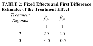
The case above demonstrates how heterogeneity can cause estimates of the average treatment effect to be negative even though the individual treatment effects are all positive. More generally, βfe will not be the same as βfd; and given heterogeneity, either one, or the other, or both can be a biased estimate of the average treatment effect on the treated (ATT).
How Do You Know If You Have a Problem?
Define ΔTR as the ATT, weighted by the number of individuals in each (g,t) cell:
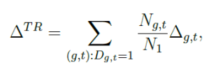
(in the example above, Ngt = 1 and N1 = 3).
βfe and βfd are also weighted measures of the ATT, but they have an additional set of weights (wgt and wfd,gt, respectively).
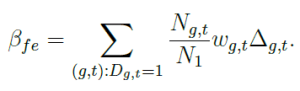
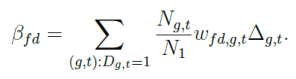
Note that βfe and βfd employ different weights wg,t and wfd,g,t. A necessary condition for both estimators to provide an unbiased estimate of ΔTR is that the weighting terms wg,t and wfd,g,t be uncorrelated with the respective treatment effects.
Thus, one diagnostic is to test for a significant difference between βfe and βfd.. If the two estimates are significantly different, that is an indicator that at least one of the two estimators is a biased estimator of the overall treatment effect.
Another diagnostic is to regress the weights on a variable that is associated with the size of the treatment effect. If one finds a significant correlation, then that is an indicator that the respective estimator (βfe or βfd.) is a biased estimator of ΔTR.
The Solution
C&D propose an estimator that focuses on treatment changes. The estimator compares treatment changes over consecutive time periods (either untreated or treated, or treated to untreated) with other observations during the same time period whose treatment did not change. They call this estimator the WTC estimator, for Wald-Time Corrected. While the example above consisted of a very restricted case (binary treatment, only one observation per (g,t) cell), their estimator generalizes to cases where treatment is continuous, and where only a portion of individuals in a given (g,t) cell receive treatment.
As a check on their estimator, they suggest a placebo estimator. The placebo estimator relates treatment changes to outcomes from the preceding period. Under the “common trends” assumption, the placebo estimator WplTC should equal zero. Failure to reject this hypothesis provides some evidence that the assumptions underlying the WTC estimator are valid.
A Replication Application
In their paper, C&D replicate results from the study, “The Effect of Newspaper Entry and Exit on Electoral Politics”, published in the American Economic Review in 2011 by Matthew Gentzkow, Jesse Shapiro, and Michael Sinkinson (GSS). GSS use county-level data from the US for the years 1868-1928 to estimate the relationship between Presidential turnout and the number of newspapers in a county. Following C&D, I explain how to implement their procedures and compare their results with those reported by GSS.
In the notation of the leading example above,
Ygt = Presidential turnout in county g at time t,
Dgt = Number of newspapers in county g at time t.
GSS use a first-difference estimator to estimate the effect of an additional newspaper on Presidential turnout. Their difference specification includes state-year fixed effects, and clusters on counties. They estimate that an additional newspaper in a county increased Presidential turnout by 0.26 percentage points (average Presidential turnout was approximately 65 percent during this period). Their estimate is reported below (cf. βfd). C&D use GSS’s data to also estimate a conventional fixed effects estimate and this is also reported in the table (cf. βfe). Note that the fixed effects estimator produces a negative estimate.

C&D first test H0: βfd = βfe and obtain a t-stat of 2.86, rejecting the null at conventional levels of significance. This indicates that at least one of these is a biased estimator of the overall treatment effect.
As a further test, C&D estimate the relationship between the respective weights, wfd,gt and wgt, and the treatment effect. Of course, the treatment effect is unobserved. As a proxy for the size of the treatment effect, C&D use year. C&D hypothesize that the effect of newspapers might change over time as other sources of communication, such as radio towards the end of the period, became more important.
To estimate this relationship, C&D employ a user-written Stata program called twowayfeweights. An example command for βfe is given below.
twowayfeweights prestout cnty90 year numdailies, type(feTR) controls(styr1-styr666) breps(100) brepscluster(cnty90) test_random_weights(year)
The command is twowayfeweights. The outcome variable is presidential turnout (prestout), the group and time variables are cnty90 and year, respectively. The treatment variable is numdailies. The option type identifies whether one is estimating weights for βfe or βfd (the syntax for βfd is slightly different). controls and breps identify, respectively, the other variables in the equation (here, state and year fixed effects), and the number of bootstrap replications to run. brepscluster indicates that the bootstrapping should be blocked according to county. The last option, test_random_weights regresses the respective weights on the variable assumed to be related to the size of the treatment effect (year). Note that while the weights are not automatically saved, there is an option to save them so that one can observe how they vary across counties and years. The results are reported below.

The results suggest that βfd may be adversely affected by correlation between the weights and the treatment effect, causing it to be a biased estimator of the overall average treatment effect on the treated. Note, however, that the sign of the correlation does not, per se, indicate the sign of the associated bias. On the other hand, the fixed effects estimator does not demonstrate evidence that the corresponding weights are correlated with treatment effects.
The last step consists of estimating the treatment effect using the WTC estimator. To do that, we use another user-written Stata program called fuzzydid:
fuzzydid prestout G_T G_T_for year numdailies, tc newcateg(0 1 2 1000) qualitative(st1-st48)
The syntax is similar to twowayfeweights, except that following the outcome variable (prestout) are two indicator variables. These indicate whether the treatment variable (numdailies) increased (G_T=1), decreased (G_T=-1) or stayed the same (G_T=0), compared to the preceding election period. G_T_for is the lead value of G_T in the immediately succeeding election period.
The options indicate that the Wald-Time Corrected statistic is to be calculated (tc), newcateg lumps the number of newspapers into 4 categories (0, 1, 2, and >2), and that state fixed effects should be included in the estimation (qualitative).
The reason for combining numbers of newspapers greater than 2 into a single category is that control groups need to have the same number of “treatments” as the treatment group. From the histogram below, it is apparent that relatively few counties have more than two newspapers.
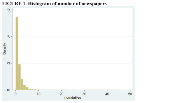
C&D estimates of the effect of newspapers on Presidential turnout are given below. They estimate an additional newspaper increases turnout by 0.43 percentage points (compared to 0.26 and -0.09 for the first-difference and fixed-effects estimators). Their placebo test produces an insignificant estimate, suggesting that the assumptions of the Wald-TC estimator are valid. Finally, as the placebo estimate uses a somewhat restricted sample, they reestimate the treatment effect on the restricted sample and obtain an estimate very close to what they obtain using the larger sample (0.0045 versus 0.0043).

Conclusion
C&D show that conventional estimates of treatment effects in two-way fixed effects models consist of weighted averages of individual treatment effects. When treatment effects are heterogeneous, this can cause conventional estimates to be biased. C&D present both (i) tests to identify if heterogeneous treatment effects present a problem for conventional estimators, and (ii) an alternative estimator that allows unbiased estimation of average treatment effects on the treated.
Replication researchers may find C&D’s procedures useful when re-analyzing original studies that estimate treatment effects within a two-way, fixed effects model.
Bob Reed is a professor of economics at the University of Canterbury in New Zealand. He is also co-organizer of the blogsite The Replication Network. He can be contacted at bob.reed@canterbury.ac.nz.
References
de Chaisemartin, C., D’Haultfœuille, X. and Guyonvarch, Y., 2019. Fuzzy Differences-in-Differences with Stata. The Stata Journal (in press).
I am a member of the Peer Reviewers Openness (PRO) Initiative. The Pro Initiative is based on the idea that reviewers have the power to get journals to become more transparent. In particular, they encourage reviewers to request data and code from the journal when they are asked to review a manuscript. Here is the statement from their homepage:
“We believe that openness and transparency are core values of science. … The promise of open research can finally be realized, but this will require a cultural change in science. The power to create that change lies in the peer-review process.”
“We suggest that beginning January 1, 2017, reviewers make open practices a pre-condition for more comprehensive review. This is already in reviewers’ power; to drive the change, all that is needed is for reviewers to collectively agree that the time for change has come.”
This can work! I was recently asked to review a manuscript for a journal that does not require authors to provide their data and code along with their manuscript at the time of submission. In other words, a typical journal. Here is what I wrote the editor:
Dear Professor XXX,
Thank you for the invitation to review a manuscript for XXX.
I am happy to do that conditional on the authors providing their data and code so I can double check their analysis.
I am a member of the Peer Reviewers’ Openness Initiative. I also co-founded and manage The Replication Network. The bottom line is that I believe that many if not most of the research findings in empirical economics are not reliable. The only way to address this problem that I can see is to have researchers provide their data and code upon submission so that reviewers can do a satisfactory job of assessing the research.
As somebody who also sits on the other side of the desk, I know how difficult it can be to secure reviewers. I don’t want to make your job more difficult than it already is. But I do think our discipline has a serious problem and I don’t know of any other way to fix it but to encourage journals to require authors to provide their data and code.
I look forward to hearing your response.
Sincerely,
Bob Reed
Frankly, I did not expect to receive a positive response from the journal, but I am apparently a man of little faith. A few days later I received the following response:
Dear Prof. Reed,
I have contacted the author and got the following reply:
“No problem. We value transparency. The data is stored on Harvard Dataverse under the link XXX (I have attached relevant information to our application, and I attach the data itself to the message for convenience). As for the code (also attached) it is designed for the R environment.
I hope this helps in assessing our findings.”
I hope that you will now be able to accept this invitation to review:
Thanks in advance.
Best regards,
XXX
As anybody knows who ever has tried to find reviewers, good reviewers are scarce. Anything that is scarce has value. And value translates to leverage. Reviewers have the leverage to get journals to become more transparent. So…why not give it a go the next time you are asked to review a manuscript?
Bob Reed is a professor of economics at the University of Canterbury in New Zealand. He is also co-organizer of the blogsite The Replication Network. He can be contacted at bob.reed@canterbury.ac.nz.
[From the blog “Registering studies when all you want is a little more credibility” by Berk Ozler, posted at World Bank Blogs]
“Some time ago, colleagues from World Bank (WB) operations contacted me with a request to evaluate an upcoming cash transfer program for refugees in Turkey.”
“With observational studies, the default mode of operation is that the researcher gets access to all the data, picks an identification strategy, does the analysis, and writes up the results. The trouble is, I do not trust myself (or my collaborator) to not be affected in our choices by the impact findings, their statistical significance, etc. … I am worried about subconscious choices that can take the analysis in one direction than the other – exactly because I can see the consequences of these choices pretty easily if I have all the data…”
“So, this is what we did: we asked the WB task team leader (TTL) to only give us the baseline data. My collaborator would then look at various options to create proper treatment and counterfactual groups using only the baseline data, after which we would register this choice – by writing up the main identification strategy and describing the analysis that would follow once we gained access to the follow-up data.”
“The idea is that once we defined who belongs in the treatment group and who in control, then we could fall back on standard operating procedures for analyzing experimental data when we received the follow-ups.”
“We now have the data from the first follow-up and analyzing attrition – in the way we specified in the PAP. Wish us luck…”
[From the article “A solution to psychology’s reproducibility problem just failed its first test” by David Adam, published at www.sciencemag.org]
“Efforts to improve the robustness of research by asking psychologists to state their methods and goals ahead of time, a process called preregistration, have stumbled at the first hurdle.”
“‘Preregistration is not as easy as it may seem,’ says Aline Claesen, a psychologist at the Catholic University of Leuven (KU Leuven) in Belgium. She and her colleagues examined 27 preregistration plans filed by psychologists from February 2015 … to November 2017. In every case, … the researchers deviated from their plan—and in every paper but one, they did not fully disclose these deviations.”
“‘I was totally surprised by how many of these [changes] were undisclosed,’ says Wolf Vanpaemel, a psychologist on the KU Leuven team. ‘There’s no good excuse for not transparently indicating all changes you made.'”
“The lack of transparency is troubling, but understandable, Vanpaemel says: Some researchers might fear their paper won’t be published if they admit to not having entirely followed their preregistration.”
“Steve Lindsay of the University of Victoria in Canada who is also editor-in-chief of Psychological Science admits that he has given authors plenty of leeway to write vague preregistrations and not account for all the deviations in a paper. He says policing the system would take time and effort the journal hasn’t budgeted for.”
“…Dan Simons, a psychologist at the University of Illinois in Champaign, describes the identified shortcomings as growing pains. ‘My guess is that most [authors] were well-intentioned and just didn’t know how to do it very well.'”
“Brian Nosek, a psychologist at the University of Virginia in Charlottesville who directs the Center for Open Science, which runs the Open Science Framework, says the KU Leuven team’s findings should help. ‘The key message here,’ he says, ‘is that preregistration is a skill and not a bureaucratic process.'”
[From the blog “Be careful what you wish for: cautionary tales on using single studies to inform policymaking” by Emmanuel Jimenez, posted at http://www.3ieimpact.org.]
“For a development evaluator, the holy grail is to have evidence from one’s study be taken up and used in policy or programming decisions that improve people’s lives.”
“In 2014, an article published in The Lancet reported the efficacy of a new vaccine, Dengvaxia, in dramatically lowering the incidence of the disease. The drug was approved in 19 countries, including the Philippines. In late 2016, the Philippines procured millions of doses and, over the span of 18-24 months, proceeded to inoculate some 800,000 school children.”
“There are now criminal charges being considered against the researcher and health officials, who sanctioned the programme. While the clinical trials were apparently well-conducted, there is doubt about how policies were drawn from them. Apparently, the vaccine, while very effective as a prophylactic for those who have already been exposed to dengue, may actually be dangerous for those who have never had it.”
“One lesson is the danger of relying on single studies to inform policy. Multiple contextual factors can influence effectiveness. To the extent possible, synthesise evidence through rigorous theory-based systematic reviews that include meta-analysis.”
“3ie is not only supporting this work but it is also facilitating access to evidence through our systematic review repository.”
“A final lesson is the importance of promoting research transparency and replications. The public inquiry into the Dengvaxia episode was prompted by a healthy scholarly debate which included policymakers. A critical aspect is the replication of scientific work. The ‘crisis’ caused by the inability to replicate some highly influential studies (including in the social sciences) is beginning to change how research is done.”


You must be logged in to post a comment.