[Excerpts taken from the working paper “Replicator Degrees of Freedom Allow Publication of Misleading “Failures to Replicate” by Christopher Bryan, David Yeager, and Joseph O’Brien, posted at SSRN]
“…using data from an ongoing debate, we show that commonly-exercised flexibility at the experimental design and data analysis stages of replication testing can make it appear that a finding was not replicated when, in fact, it was.”
“The present analysis is important, in part, because it provides the sort of direct demonstration that has the potential to spur change.”
“We focus here on the debate about whether a subtle manipulation of language—referring to voting in an upcoming election with a predicate noun (e.g., “to be a voter”) vs. a verb (e.g., “to vote”)—can increase voter turnout.”
“A preliminary analysis of the data from just the day before the election revealed that many of the most obvious model specifications yielded significant replications of the original noun-vs.-verb effect.”
“A closer examination of the analyses reported by Gerber and colleagues (35) in support of their claim of non-replication revealed that the replicating authors chose to include three features…that in combination are known to increase the risk of misleading results.”
“…study results often hinge on data analytic decisions about which reasonable and competent researchers can disagree…we employed an analytical approach that is expressly designed to provide a comprehensive assessment of whether study data support an empirical conclusion when the influence of arbitrary researcher decisions on results is minimized.”
“The primary statistical approach we employ, called “Specification-Curve Analysis,” involves running all reasonable model specifications (i.e., ones that are consistent with the relevant hypothesis, expected to be statistically valid, and are not redundant with other specifications in the set…”
“An associated significance test for the specification curve, called a “permutation test,” quantifies how strongly the specification curve as a whole (i.e., all reasonable model specifications, taken together) supports rejecting the null hypothesis.”
“The results … make clear that noun wording had a significant effect on turnout overall…But the specification curve results also strongly suggest that the replicating authors’ data analysis choices might not be the only replicator degree of freedom influencing results. Rather, a design-stage degree of freedom exercised by the replicating authors, regarding the window of time in which the study was conducted, may have further driven the treatment effect estimate downward…”
“Perhaps the clearest, most concrete implication of the present analysis is that specification-curve analysis should be standard practice in replication testing.”
To read the full paper, click here.
[Excerpts taken from an email sent out by the American Economic Association to its members on July 16, 2019]
“On July 10, 2019, the Association adopted an updated Data and Code Availability Policy, which can be found at https://www.aeaweb.org/journals/policies/data-code. The goal of the new policy is to improve the reproducibility and transparency of materials supporting research published in the AEA journals.”
“What’s new in the policy?”
“A central role for the AEA Data Editor. The inaugural Data Editor was appointed in January 2018 and will oversee the implementation of the new policy.”
“The Data Editor will regularly ask for the raw data associated with a paper, not just the analysis files, and for all programs that transform raw data into those from which the paper’s results are computed.”
“Replication archives will now be requested prior to acceptance, rather than during the publication process after acceptance…”
“There is a new repository infrastructure, hosted at openICPSR, called the “AEA Data and Code Repository.” Data (where allowed) and code (always required) will be uploaded to the repository and shared with the Data Editor prior to publication.”
“The Data Editor will assess compliance with this policy and will verify the accuracy of the information.”
“Will the Data Editor’s team run authors’ code prior to acceptance? Yes, to the extent that it is feasible. The code will need to produce the reported results, given the data provided. Authors can consult a generic checklist, as well as the template used by the replicating teams.”
“Will code be run even when the data cannot be posted? This was once an exemption, but the Data Editor will now attempt to conduct a reproducibility check of these materials through a third party who has access to the (confidential or restricted) data.”
[From the blog “Pre-results Review at the Journal of Development Economics: Lessons learned so far” by Andrew Foster, Dean Karlan, Edward Miguel and Aleksandar Bogdanoski, posted at Development Impact at World Bank Blogs]
“In March 2018, the Journal of Development Economics (JDE) began piloting Pre-results Review track (also referred to as “registered reports” in other disciplines) in collaboration with the Berkeley Initiative for Transparency in the Social Sciences (BITSS).”
“The motivation behind this exercise was simple: both science and policy should reward projects that ask important questions and employ sound methodology, irrespective of what the results happen to be.”
“A little over one year in, we reflect on the experience so far and offer our perspectives on the future of pre-results review at the JDE and in the discipline as a whole.”
“What we’ve learned so far”
“Referees (and editors) have found it hard on several occasions to judge submissions … not knowing the final results…”
“Work should be submitted relatively early for two reasons: (a) to maximize the possibility that feedback can be used in shaping final data collection, and (b) to ensure enough time for an R&R round and resubmission before the final data come in. This means at a minimum of three months, but ideally six months to a year, before data collection of the key outcome data.”
“Many authors have found Pre-results Review helpful in improving the ultimate quality of their research papers.”
“Reasons for rejection in Pre-results Review are similar to those in the regular review process.”
“We expected that the existence of a pre-results review submission track would eventually incentivize researchers to take on projects that they perceive as risky …our initial impression is that the Stage 1 submissions to the JDE so far do not appear to be substantially more (or less) risky than papers submitted through the normal journal review track.”
“Stage 2 of review at the JDE will likely allow for some flexibility in interpreting deviations from research designs accepted at Stage 1. This flexibility may be at odds with emerging best practices in other disciplines.”
“…because field experiments study human interactions in a real-world context, precautions need to be taken to prevent biasing participants’ behavior. …This means that we may not always be able to fully publicize accepted Stage 1 proposals until fieldwork is completed, even though this may be at odds with what is recommended in other disciplines…”
“…since development economics experiments can literally take years before data collection is complete, it may also be a while before the JDE is able to publish the first paper in the pre-results review track.”
To read more, click here.
[* EiR = Econometrics in Replications, a feature of TRN that highlights useful econometrics procedures for re-analysing existing research. The material for this blog is drawn from a recent working paper, “On the measurement of importance” by Olivier Sterck.]
NOTE: The files (Stata) necessary to produce the results in the tables below are posted at Harvard’s Dataverse: click here.
Researchers are often interested in assessing practical, or economic, importance when doing empirical analyses. Ideally, variables are scaled in such a way that interpreting a variable’s effect is straightforward. For example, a common variable in cross-country, economic growth equations is average annual temperature. Accordingly, one can gauge the effect of a 10-degree increase in temperature on economic growth, ceteris paribus.
However, sometimes variables do not allow a straightforward interpretation. This is true, for example, for index variables. It is also true for variables that are otherwise difficult to relate to, such as measures of “terrain ruggedness” or “genetic diversity”, both of which have been employed in growth studies.
Problems can still arise even when coefficients are straightforward. For example, a variable may have a large effect, but differ only slightly across observations, so that it explains very little of the variation in the dependent variable.
Further, a researcher may be interested in assessing the relative importance of variables. For example, the coefficients on average annual temperature and percentage of fertile soil may be straightforward to interpret, but a researcher may be interested knowing which is “more important” for explaining differences in growth rates across countries.
The most common approach for measuring importance in these latter cases is to calculate Standardized Beta Coefficients. These are obtained by standardizing all the variables in an equation, including the dependent variable, and re-running the regression with the standardized variables. However, this measure has serious shortcomings.
As we shall show below, the nominal value of the Standardized Beta Coefficient does not lend itself to a straightforward interpretation. Further, it has difficulty handling nonlinear specifications of a variable, such as when both a variable and its square is included in an equation. And it is unable to assess groups of variables. For example, a researcher may include regional variables such as North America, Latin America, Middle East, etc., and wish to determine if the regional variables are collectively important.
A recent paper by Olivier Sterck identifies shortcomings of existing measures of importance (such as the Standardized Beta Coefficient) and proposes two new measures: Ceteris Paribus Importance and Non-Ceteris Paribus Importance. Both are measured in percentages and have straightforward interpretations. They can be implemented with a new Stata command (“importance”) that can be downloaded from the author’s website. The two measures address different aspects of importance and are intended as complements.
Ceteris Paribus Importance
Let the relationship between a variable of interest, y, and a set of explanatory variables be given by
(1) yi = b0 + ∑i bixi + εi
It follows that the variance of y is
(2) Var(y) = ∑i=1/n Var(bixi) + 2∑i=1/n-1∑j=i+1/n Cov(bixi,bjxj) Var(ε) .
A key challenge is how to allocate the Cov(bixi,bjxj) terms between xi and xj for all i ≠ j. The first measure, Ceteris Paribus Importance, denoted qi-squared, addresses this problem by ignoring these terms:
(3) qi-squared = Var(bixi) / [∑i=1/n Var(bixi) + Var(ε)]
Ceteris Paribus Importance takes values between 0 and 1 and can be understood as a percentage. Specifically, it is the percent of variation in y attributed to a given variable, holding the other variables constant. Note that the sum of the individual q-squared terms, including q-squared for the error term, equals one: ∑i=1/n qi-squared + q-squared(ε) = 1. Further, in the special case when ∑i=1/n-1∑j=i+1/n Cov(bixi,bjxj) = 0, as when all the explanatory variables are uncorrelated with each other, ∑i=1/n qi-squared = R2.
A comparison of Ceteris Paribus Importance with Standardized Beta Coefficient
Consider two data generating processes (DGPs).
DGP1: y1i = x1i + ε1i , where x1i, ε1i ~ N(0,1);
DGP2: y2i = x2i + ε2i , where x2i ~ 2·N(0,1) and ε1i ~ N(0,1).
In the first DGP, the coefficient on x1i is 1 and x1i and ε1i each contribute 50% to the variance of y. The second DGP is identical to the first, except that x now contributes 80% of the variance of y. The table below reports coefficient estimates for both models from simulated samples of 10,000 observations. It also reports the corresponding Ceteris Paribus Importance (qi-squared) and Standardized Beta Coefficient measures.

Recall that Ceteris Paribus Importance measures the contribution of the x variable to the variance of y. Since there is only one explanatory variable in both DGPs, the covariance terms in equation (3) drop out, and qi-squared = R-squared. Accordingly, in DGP1, where both x and ε contribute equally to the variance of y, Ceteris Paribus Importance equals 50%. When the variance of x increases fourfold, so that x contributes 4/5s of the variance of y, Ceteris Paribus Importance rises to 80%. In both cases, Ceteris Paribus Importance has a straightforward interpretation as a percent of the variance of y contributed by x (holding other variables constant).
The corresponding Standardized Beta Coefficients for the two models are 0.714 and 0.894. While the Standardized Beta Coefficient is larger in the second model, there is no straightforward interpretation of its numerical value.
Non-Ceteris Paribus Importance
Sterck’s second measure, Non-Ceteris Paribus Importance, accommodates the fact that variables are likely to be correlated when working with observational data. It allocates the covariance terms in equation (2) equally across the two variables and is defined as follows:
(4a) Ei = [Var(bixi) / Var(y)] + [∑j≠i/n Cov(bixi,bjxj) / Var(y)].
This can be expressed alternatively as
(4b) Ei = [∂Var(y)/Var(y)] / [∂Var(bixi)/Var(bixi)] .
Despite its seemingly nonintuitive appearance, Non-Ceteris Paribus Importance has two characteristics that make it appealing. First,∑i=1/n Ei = R-squared. Thus, it decomposes R-squared across the respective variables. As shown by equation (4.b), the individual components can be expressed as elasticities. In particular, they measure how a marginal change in the variance of bixi affects the variance of y.
The second characteristic is that Non-Ceteris Paribus Importance can take both positive and negative values. The first term in equation (4), [Var(bixi) / Var(y)], will always be positive, of course. However, the second term captures the association of xi with the other explanatory variables. In particular, if xi is strongly negatively correlated with other variables, the overall effect of increases in the variance of bixi can be to decrease the variance of y.
Non-Ceteris Paribus Importance serves as a complement to Ceteris Paribus Importance. The latter focuses on the direct effect of x on the variance of y. In contrast, Non-Ceteris Paribus Importance incorporates the covariance of xi with other variables. It provides a measure of the extent to which xi works to reinforce, or counteract, the effects of the other explanatory variables.
An application to growth empirics
Sterck provides an empirical example of the two importance measures using income data from 155 countries. He employs OLS to estimate a regression of the log of per capita GDP in 2000 on 18 variables that have been used by other researchers of economic growth.
Table 2 classifies the variables in five groups. Category 1 consists of stand-alone variables. Category 2 consists of a quadratic specification for the variable Predicted genetic diversity. Categories 3 through 5 consist of groupings of dummy variables (religion, legal foundations, regions).
Note that Standardized Beta Coefficients are unable to collectively evaluate Categories 2 through 5. For example, one can calculate a Standardized Beta Coefficient for the linear and quadratic forms of the Predicted genetic diversity variable, but not for their combined importance. Likewise, one can calculate Standardized Beta Coefficients for the individual religion dummies, but one cannot use this measure to obtain an overall measure of the importance of religion.

Table 3 reports importance measures for the 5 categories of variables (where the stand-alone variables of Category 1 are lumped together for convenience).

Column (1) displays Ceteris Paribus Importance (qi-squared). Note that the importance of the individual categories plus the residuals sum to 100 percent of the variance of y. Corporately, the stand-alone variables account for approximately 45% of the variance of y, with the religion and regional variables next in importance at 13% and 10%, respectively.
Column (2) reports Non-Ceteris Paribus Importance (Ei). This measure accounts for the interactions of variables across categories. The individual shares sum to the R-squared of the respective OLS regression (84.4%).
Columns (3) and (4) divide Non-Ceteris Paribus Importance into two components. The Variance and Covariance components correspond to the first and second terms in equation (4.a) above. In most cases, variables within a category reinforce the effects of variables in other categories. However, note that the Covariance term for the regional variables is negative. This indicates that the regional dummies counteract the effect of some of the variables in other categories, reducing the variation of y that would otherwise result. Nevertheless, overall, regional variables positively contribute to the variance of incomes across countries.
The above provides an example of how Ceteris Paribus and Non-Ceteris Paribus Importance can be calculated for OLS regressions. An option in the corresponding do file also allows one to calculate importance measures for 2SLS regressions. Additional details are provided in Sterck’s paper.
Bob Reed is a professor of economics at the University of Canterbury in New Zealand. He is also co-organizer of the blogsite The Replication Network. He can be contacted at bob.reed@canterbury.ac.nz.
[From the article “Certify reproducibility with confidential data” by Christophe Pérignon, Kamel Gadouche, Christophe Hurlin, Roxane Silberman, and Eric Debonnel, published in Science]
“Many government data, such as sensitive information on individuals’ taxes, income, employment, or health, are available only to accredited users within a secure computing environment…However, researchers using confidential data are inexorably challenged with regard to research reproducibility.”
“We describe an approach that allows researchers who analyze confidential data to signal the reproducibility of their research. It relies on a certification process conducted by a specialized agency accredited by the confidential-data producers and which can guarantee that the code and the data used by a researcher indeed produce the results reported in a scientific paper.”
“In France, the Centre d’Accès Sécurisé aux Données (CASD) is a public research infrastructure that allows users to access and work with government confidential data under secured conditions. This center currently provides access to data from the French Statistical Institute and the French Ministries for Finance, Justice, Education, Labor, and Agriculture, as well as Social Security contributions and health data.”
“The Certification Agency for Scientific Code and Data (cascad, http://www.cascad.tech) is a not-for-profit certification agency created by academics…cascad was granted a permanent accreditation by the French Statistical Secrecy Committee to all 280 datasets available on CASD…the whole certification process remains within the CASD environment…no data can ever be downloaded.”
“When an author requests a cascad certification for a paper, he or she needs to provide the paper, the computer code used in the analysis, and any additional information (software version, readme files, etc.) required to reproduce the results. Then, a reproducibility reviewer, who is a full-time cascad employee specialized in the software used by the author, accesses a CASD virtual machine that is a clone of the one used by the author.”
“The reviewer executes the code, compares compares the output with the results displayed in the tables and figures of the paper, and lists any potential discrepancies in an execution report…a reproducibility certificate is sent to the author and is stored in the cascad database…The author can transfer the reproducibility certificate to an academic journal when submitting a new manuscript.”
To read the full article, click here. (NOTE: The article is behind a paywall.)
[From the article “The standard errors of persistence” by Morgan Kelly, published at Vox – CEPR Policy Portal]
“Does the slave trade continue to affect trust between people in Africa? Does a country’s prosperity depend on the genetic diversity of its population? Do arbitrary colonial boundaries continue to drive poverty in Peru and internal conflict in Africa? These and other questions are part of a substantial literature on persistence, or deep origins, which finds that many modern outcomes strongly reflect the characteristics of the same place in the more or less distant past.”
“While a judicious choice of variables or time periods might coax a t statistic towards 1.96, there would seem to be no way that the t statistics of four, five, or even higher that appear routinely in this literature could be the result of massaging regressions …”
“Such persistence results must instead reflect … the enduring legacies of the past. However, alongside unusually high t statistics, persistence regressions usually display extreme levels of spatial autocorrelation of residuals.”
“Figure 1 gives the basic idea. I generate two spatial noise series – where areas with high values are coloured yellow and those with low values purple – and take their values at the white dots which correspond to towns. I will call one noise series the ‘modern’ outcome (say, GDP per capita or attitudes toward immigrants), and the other I label the ‘historical’ variable (say, deaths in the Thirty Years’ War or duration of rule by the Ottoman Empire).”
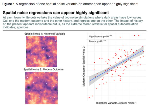
“If you regressed one variable on the other without knowing that they are both artificial noise, you would probably conclude from Figure 1 that the ‘historical’ variable exerts an overwhelming impact on the ‘modern’ outcome.”
“…there turns out to be a reliable indicator to caution us that our findings may be specious, and that indicator is the Moran statistic. The Moran statistic is the standard test for spatial autocorrelation in regression residuals … No study that I examine below reports Moran statistics.”
“I analyse the results of 28 persistence papers that have appeared in the American Economic Review, Econometrica, Journal of Political Economy, and Quarterly Journal of Economics to assess their robustness to spatial noise. The approach is to replicate the first substantive regression of the paper …”
“The Z scores of Moran statistics for each regression are shown in Figure 2 and we can see that, with some exceptions, the spatial autocorrelation in these results is extreme.”
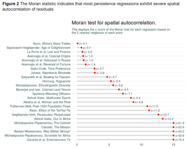
“…we have seen that a standard Moran statistic serves as a useful warning light for potential trouble with spatial noise. My results suggest that in cases where this statistic is not reported the findings of persistence studies (and regressions using spatial data more generally) should be treated with some caution.”
[From the working paper, “Lagged Variables as Instruments” by Yu Wang and Marc Bellemare, posted at http://www.marcfbellemare.com]
“…applied econometricians often settle on less-than-ideal IVs in an effort to “exogenize” x … One such less-than-ideal identication strategy is the use of what we refer to throughout this paper as a ‘lagged IV’.”
“… a lagged IV entails using a lag xi,t-1 … as an IV for xit. The argument that is typically (and often implicitly) made in such cases is that since xi,t-1 precedes xit in time, the causality runs entirely from xi,t-1 to xit, and since there is presumably a high degree of autocorrelation in x, xi,t-1 should be a valid IV for xit.”
“In this paper, we look at the consequences of a lagged IV on the bias of the estimated coefficient …, its root mean squared error (RMSE), and on the likelihood of making a Type I error … We first do so analytically, which allows identifying the precise conditions under which one can use a lagged IV. … We next use Monte Carlo simulations to show what happens to bias, RMSE, and the likelihood of a Type I error for a broad range of the relevant parameters.”
“…we find that if the lagged IV xi,t-1 has no direct causal impact (i) on the dependent variable nor (ii) on the unobserved confounder, it … can mitigate the endogeneity problems by reducing bias and the root mean square error (RMSE) relative to OLS … however, the likelihood of a Type I error remains large.”
“On the other hand we find that if the lagged IV xi,t-1 has a direct causal impact (i) on the dependent variable, on (ii) on the unobserved confounder, or both, … a lagged IV worsens the endogeneity problem by increasing bias as well as the RMSE relative to OLS. Moreover, in such cases, the likelihood of Type I error is almost always equal to one for common ranges of parameter values.”
“In practical terms, this means that the use of a lagged IV often leads one to report coefficient estimates of questionable economic significance (because of the increased bias) and statistical significance (because of the greater likelihood of a Type I error). Worse, the use of lagged IVs will tend to lead one to conclude that a causal relationship exists where it does not.”
“Suppose we have the structural equation
(1) yit = b xit + θ xi,t-1 + δ uit + εit ,
where y, x, and ε respectively denote the dependent variable, the variable of interest and an error term … but where u denotes confounders.”
“We specify two autocorrelation functions: one for x, and one for u, such that
(2) xit = ρ xi,t-1 + κ uit + ηit , and
(3) uit = φ ui,t-1 + ψ xi,t-1 + υit .”
“Using the framework laid out in equations (1), (2), and (3), we can explore four distinct endogeneity scenarios:”
“1. θ = 0 and ψ = 0, i.e., the lagged variable of interest has no direct causal impact on the dependent variable, nor does it have a causal impact on the unobserved confounder.”
“2. θ ≠ 0 and ψ = 0, i.e., the lagged variable of interest has a direct causal impact on the dependent variable, but it does not have a causal impact on the unobserved confounder.”
“3. θ = 0 and ψ ≠ 0, i.e., the lagged variable of interest has no direct causal impact on the dependent variable, but it has a causal impact on the unobserved confounder.”
“4. θ ≠ 0 and ψ ≠ 0, i.e., the lagged variable of interest has a direct causal impact on the dependent variable, and it has a causal impact on the unobserved confounder.”
“In scenario 2, since θ ≠ 0, xi,t-1 directly influences yit via its marginal effect θ.”
“In Scenario 3, although θ = 0, ψ ≠ 0, and xi,t-1 still influences yit via marginal effect θψ, derived from equations (2) and (3). Therefore, both scenario 2 and 3 violate not only the independence assumption, but also the exclusion restriction, and so they will result in biased estimates.”
“A similar result obtains for scenario 4, which is just a combination of the undesirable features (i.e., θ ≠ 0 and ψ ≠ 0) in scenarios 2 and 3.”
“Since in scenario 3, xi,t-1 has a direct impact on uit, which could include more than one unobserved covariate, it implies that xi,t-1 could have more than one causal path whereby it influences yit.”
“…even if theoretical arguments state that the lagged variable of interest has no direct impact on the dependent variable—in other words, even if those arguments make the case that scenario 2 does not hold—it is difficult to argue against the possible existence of scenarios 3 and 4, which both results in a violation of the exclusion restriction.”
“Turning to scenario 1, although the lagged IV in this case has neither a direct causal impact on the dependent variable nor on the unobserved con-founder, the lagged IV may still indirectly be correlated with the dependent variable. Specifically, since ui,t−1 influences both uit and ui,t−1, xi,t-1 and uit have a simultaneous relationship.”
“In other words, as xi,t-1 changes, uit changes contemporaneously (albeit not causally), and so yit changes as well. In this case although xi,t-1 influences yit only through xit, which satisfies the exclusion restriction, the IV xi,t-1 violates the independence assumption because it does not serve as a random exogenous shock.”
“…the independence assumption can only be satisfied by assuming that there are no dynamics among unobserved confounders (Bellemare et al. 2017). Therefore, even if the dynamic causal impacts are restricted and thus exclusion restriction is satisfied, a lagged IV can still be problematic because of the unavoidable violation of independence assumption that it entails.”
“The implications of our findings for the practice of applied econometrics are obvious. Unless one can make the claim that both the independence assumption and the exclusion restriction hold, lagged IVs should be avoided in the name of bias, RMSE, and the likelihood of a Type I error. But given that the independence assumption requires that one make the dubious assumption that there are no dynamics among unobserved confounders, this essentially means that lagged IVs should be avoided entirely.”
To read the article, click here.
[From the commentary “Novelty in science should not come at the cost of reproducibility” by Andrew Holding, published in The FEBS Journal]
“Oestrogen receptor (ER) cycling is a dogma of the Oestrogen receptor-positive (ER+) breast cancer field.”
“For nearly 20 years, it was accepted dogma that, once stimulated, the ER activated its target genes in successive 90-min ‘on–off’ cycles … The papers that first detailed this process currently have over 1000 citations each, yet we could not replicate their key findings.”
“It would be surprising if no one else had encountered this replication problem over the past two decades. …the real underlying problem here is that negative results are often not published.”
“We need to challenge the culture of ‘first past the post’ and the pre-eminence given to high-impact journal publications. Instead, we need to develop a research culture in which research outcomes are only seen as being groundbreaking once they have been independently validated.”
“In such a culture, those who replicate research findings are seen as being an important part of the research process – as important as those who got there first. In my case, so few had the time and resources to challenge the established fact that they simply published the next novel result without ensuring the underlying model was right.”
[From the preprint “Accumulation bias in meta-analysis: the need to consider time in error control” by Judith ter Schure and Peter Grünwald, posted at arXiv.org]
“Studies accumulate over time and meta-analyses are mainly retrospective. These two characteristics introduce dependencies between the analysis time, at which a series of studies is up for meta-analysis, and results within the series.”
“Dependencies introduce bias — Accumulation Bias — and invalidate the sampling distribution assumed for p-value tests, thus inflating type-I errors.”
“…by using p-value methods, conventional meta-analysis implicitly assumes that promising initial results are just as likely to develop into (large) series of studies as their disappointing counterparts. Conclusive studies should just as likely trigger meta-analyses as inconclusive ones. And so the use of p-value tests suggests that results of earlier studies should be unknown when planning new studies as well as when planning meta-analyses.”
“Such assumptions are unrealistic… ignoring these assumptions invalidates conventional p-value tests and inflates type-I errors.”
“… we argue throughout the paper that any efficient scientific process will introduce some form of Accumulation Bias and that the exact process can never be fully known.”
“A likelihood ratio approach to testing solves this problem … Firstly, it agrees with a form of the stopping rule principle … Secondly, it agrees with the Prequential principle … Thirdly, it allows for a betting interpretation …: reinvesting profits from one study into the next and cashing out at any time.”
“This leads to two main conclusions. First, Accumulation Bias is inevitable, and even if it can be approximated and accounted for, no valid p-value tests can be constructed. Second, tests based on likelihood ratios withstand Accumulation Bias: they provide bounds on error probabilities that remain valid despite the bias.”
[From the paper “Calibrating the scientific ecosystem through meta-research” by Tom Hardwicke, Stylianos Serghiou, Perrine Janiaud, Valentin Danchev, Sophia Crüwell, Steven Goodman, and John Ioannidis, forthcoming in Annual Review of Statistics and Its Application]
“Meta-research has been defined as ‘the study of research itself: its methods, reporting, reproducibility, evaluation, and incentives.'”
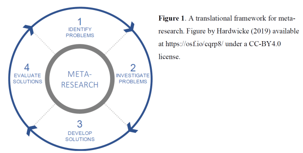
“We will map the endeavor of meta-research using the translational framework depicted in Figure 1. This framework is not necessarily comprehensive and aims to be descriptive rather than prescriptive. The goal is to highlight how individual meta-research projects form part of a broader effort to continuously calibrate the scientific ecosystem towards higher standards of efficiency, credibility, and quality.”
Outline
1. IDENTIFYING PROBLEMS
1.1 Incentives and norms
1.2 Lack of transparency
1.3 Statistical schools of thought and statistical misuse
1.4 Reproducibility
2. INVESTIGATING PROBLEMS
2.1 Incentive structures
2.2 Publication bias and selective reporting
2.3 Transparency of research resources
2.4 Suboptimal research design
2.5 Statistical misuse
2.6 Reproducibility
3. DEVELOPING SOLUTIONS
3.1 Journal, funder, society and university policies
3.2 Pre-registration and registered reports
3.3 Reporting guidelines
3.4 Peer review
3.5 Collaboration
3.6 Statistical reform
3.7 Evidence synthesis
4. EVALUATION SOLUTIONS
4.1 Journal policy
4.2 Reporting guidelines
4.3 Pre-registration and registered reports
To read the article, click here.

You must be logged in to post a comment.